


an118: Strain Gage Signal Conditioner
Application Note
Preamble
The most dominant application of bridge circuits is in the instrumentation arena. Within these applications, the strain gage as a resistive element sensitive to displacement has been used extensively for a century. Today, process variables such as load weight, pressure, flow, distance, motion, vibration, etc., employ strain gage bridge circuits as the fundamental sensor device. In addition, commercially available individual strain gage elements are combined with bridge circuit signal conditioning modules (SCMs) in custom instrumentation applications, such as structural beam deflections, internal strain within concrete structures, etc. There are scores of strain gage manufacturers with a wide spectrum of configurations for various applications. The reader is encouraged to examine strain gage manufacturers’ product specifications for more in-depth information on strain gage construction and specification details.Examining all types of individual strain gage element configurations is beyond the scope of this application note; however, the behavior fundamentals of strain gages interfaced to Dataforth’s strain gage bridge signal conditioning modules will be examined. The effects of line resistance, strain gage parameter tolerances, and methods of excitation are included.
This application note is based on the basic bridge circuit fundamentals published in Dataforth’s Application Note AN117 “Basic Bridge Circuits,” which should be considered prerequisite reading; see Reference 1.
Review Conductive Resistance
The reader is encouraged to visit Dataforth’s Application Note AN105 (Reference 2) for the simple derivation of conductive current. Conductive current, “i,” is defined as coulombs/second, the flow of charged particles as shown in Equations 1 and 2.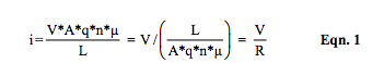
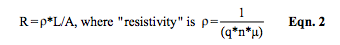
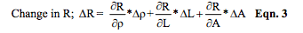
The expression for resistance, Equation 2, shows that conductive resistance depends on geometry (length and area) and the molecular structure quantities: “n,” density of electrons available for motion; “q,” charge of an electron, and “μ ,” mobility of electrons. Electron charge “q” is constant; “free” electrons “n” are dependent upon temperature and internal molecular structure, and mobility “μ ,” the relative ease with which electrons can navigate through a molecular structure, is very sensitive to temperature, material composition, and structure deformity. Mathematically (a little calculus here), the change in conductive resistance is described in Equation 3, which again says resistance change is a function of both geometry and electron behavior.
Basic Strain Gage
The following resistive strain gage element fundamentals are based on the simple element geometry of length, “L,” and cross sectional area A=x*y where the x and y dimensions are much less than L. See Figure 1.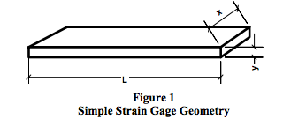
Resistive metal alloy strain gages are typically constructed in a thin foil configuration with a length considerably longer than the area dimensions. This type of strain gage can measure a change in the surface length of a test structure by bonding the gage to the surface of the test structure with an orientation such that changes in the strain gage length dimension represent the change in the surface length of the test structure. Manufacturers of strain gages have developed strain gage elements with many different configurations to facilitate sophisticated precision measurements. Readers planning to measure strain should consult strain gage manufacturers’ specifications and their product application data. The focus of this application note is limited to examining the electrical behavior of typical strain gages interfaced to Dataforth’s strain gage bridge signal conditioning modules.
Equation 4 is the result of combining Equations 2 and 3, assuming a resistive element of length, L, with area A=x*y. This expression shows how the incremental change in resistance is related to both dimensional and molecular structure changes.
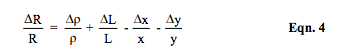
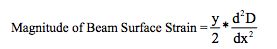
Strain “ε” in a specific dimension is defined as the incremental change in the length dimension divided by the unstressed length dimension. For example, Δ L/L in Equation 4 is the strain in the length dimension. In this example, longitudinal strain is εL = Δ L/L and transversal strain εt = (- Δ y/y) and (- Δ x/x).
In general, when a resistive element of length, L, and area, A=x*y, is stretched in the L direction, the area will tend to shrink; consequently, the incremental change in both the x and y dimensions is negative, decreasing. Over 150 years ago, Simeon Denis Poisson showed that uniaxial longitudinal strain, Δ L/L, is related to transversal strain, Δ x/x and Δ y/y, by a ratio for a given material. Poisson’s ratio is defined in Equation 5.
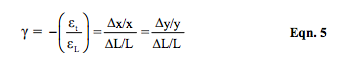
Note that Δ L is positive but Δ x and Δ y are negative.
The gage factor, GF, for a strain gage defines the relationship between resistance changes and element elongation (strain) as defined in Equation 6 by combining Equations 4 and 5.
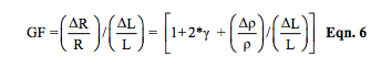
It is important to observe that gage factors of strain gages are dependent upon Poisson’s ratio and the material’s molecular structural behavior. For ideal metal alloy type strain gages, distorted elements would have minimum to no change in resistivity “ρ ” and no change in volume, resulting in an ideal magnitude limit for Poisson’s ratio of 1/2. In most alloy strain gages, Poisson’s ratio is in the range of 0.2 to 0.4. Considering the ideal case, the gage factor, GF, is 2. Table 1 illustrates some GF values for different materials.
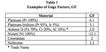
The term (Δρ /ρ ) in Equation 6 shows us that gage factors can be sensitive functions of temperature, molecular composition, and deformation. Special semiconductor strain gages with selective additives can have GFs much larger than metal alloy strain gages. Table 2 represents typical foil strain gage parameters.
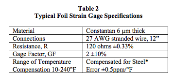
* Strain gauge manufacturers can provide temperature compensated strain gage elements that correct thermal expansions caused by the material to which a strain gage is attached. For example, steel has a coefficient of thermal expansion of ~6ppm/°F, which means a 100°F change would cause an uncompensated 600 microstrain error, or 1200ppm error in (ΔR/R) for GF = 2.
Example of Measuring Beam Bending
The following examples explore different strain gage bridge circuit topologies for measuring deflection and strains of the beam configuration illustrated in Figure 2. The strain gage instrumentation methods applied to the beam illustrated in Figure 2 are presented as examples for exploring electrical behavior of various strain gage bridge circuit topologies. This particular beam example is not a Dataforth recommendation for fixed beam strain gage instrumentation. The objective of these topology examples is to examine electrical behavior and associated errors when interfacing these circuit topologies with Dataforth’s strain gage bridge SCMs. The basic strain gage specified in Table 2 is used throughout these examples.The fixed beam configuration detailed in Figure 2 is a rectangular steel tube beam 12 feet long with a cross sectional area 2 inches wide by 4 inches vertical depth. Wall thickness of this tube is 3/16 inch. Beam ends are welded to stationary fixtures and a load density, “w,” of 500 pounds per foot is distributed over the beam’s length. Envision this structure as a support beam for a loading platform. Equations for this beam’s deflection and strain are based on approximate first order theory and are limited to uniaxial longitudinal strain and stress.
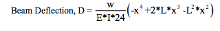
E = Modulus of Elasticity; I = Beam’s Moment of Inertia (“I” calculated via difference of rectangles)
The effects of transverse shear stress have been neglected. See Reference 3 for mathematical details.
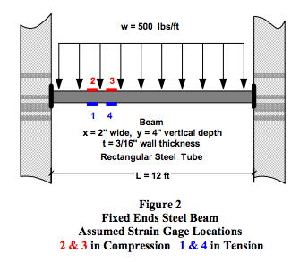
Figure 3 is a Matlab program graph, which predicts both beam deflection and bottom surface beam strain for the steel beam shown in Figure 2. The modulus of elasticity, E, is assumed to be 29E6 psi. Readers interested in reviewing the mechanics of materials will find Reference 3 to be a valuable resource.
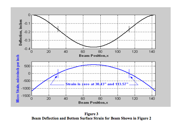
For this beam loading example, Figure 3 not only illustrates the predicted values of deflection and strain but also indicates the beam positions where surface strain is zero. Figure 3 shows the following:
- The displacement and associated strain are all symmetrical about the beam’s center.
- The bottom surface of each beam end is in compression, strain is negative, i.e., length tends to decrease.
- The bottom surface of the beam near the center is in tension, strain is positive, i.e., length tends to increase.
- At two locations equidistant from the beam center, the strain changes direction (from compression to tension) and is zero.
- Absolute strain is maximum at each end of the beam where the welds could be subject to failure. Note: The Matlab program for Figure 3 gives the magnitude of bottom surface strain at each beam end (L=0 and L=144) of 1175E-6 in/in. This strain, with an assumed modulus of elasticity, E, of 29E6 μ in/in, predicts a maximum magnitude of stress in the steel at these ends of 34.1E3 (σ = E*ε) psi. A stress of this magnitude in the steal beam ends represents a stress that is considered much too close to the yielding point for mild steel. Certainly, a strain gage instrumentation warning system on this beam may be justifiable.
Instrumentation Configuration Options
The following list identifies just some of the basic concerns that must be resolved in order to facilitate a strain gage instrumentation system.- What information is required?
- Where should the strain gage be placed to yield the required information?
- What accuracy is necessary?
- Which type bridge configuration should be selected: quarter, half, or full bridge circuit topology in Category 1 or in Category 2? See Dataforth’s Application Note AN117, Reference 1.
- Which type of excitation, voltage or current?
- Can the excitation line resistance be neglected?
- Should Category 2 type topologies be implemented with 2-wire or 3-wire field wiring?
The following options are examined as illustrative guidelines. Dataforth is not in a position to make any definitive recommendations on measuring strain, since each application is dependent upon the customer’s unique system requirements and engineering policies.
Throughout the following option examples, it is assumed that the instrumentation objective is to implement a warning system that provides an indication when the beam stress on the end welds approaches a predetermined safety limit.
Option 1: Category #1 Bridge Topology
Figure 4 illustrates the basic Category #1 R-Bridge Topology including voltage output and excitation line resistances. All bridge elements are located remote from the signal conditioning module (SCM). In the absence of process variables, R1=R2=R3=R4 defined as =R.
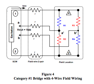
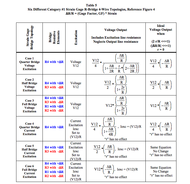
Table 5 in the Appendix illustrates output voltage expressions for six different configurations of the bridge circuit shown in Figure 4, where the resistive bridge elements exposed to beam strain are located as shown in Figure 2. In all cases, the output voltage line resistance is ignored as justified in Reference 1.
- Quarter Bridge: Case 1 and Case Bridge elements R1, R2, and R3 are fixed equal to R The strain gage element is R4 and is located as show in Figure 2.
- Half Bridge: Case 2 and Case 5 Bridge elements R1 and R2 are fixed equal to R. The strain gage elements are R3 and R4 and are located as shown in Figure 2.
- Full Bridge: Case 3 and Case 6 The strain gage elements are R1 and R2 and R3 and R4 and are located as shown in Figure 2.
NOTE: Current excitation as shown for Cases 4, 5, and 6 in Appendix Table 5 for the Category #1 bridge topologies of Figure 4 totally eliminates the effects of excitation line resistance.
Option 2: Category #2 Bridge Topology
Figures 5 and 6 illustrate the basic Category #2 R-Bridge Topology including voltage output and excitation line resistances. Bridge elements exposed to process variables are remotely located from the SCM. Bridge completion resistors R1 and R2 are included in the SCM and are equal fixed values that force Va to be equal to one-half of V12, the excitation voltage. Resistors R1 and R2 do not appear in the voltage output expressions. In the absence of process variables, R3 = R4 defined as = R.
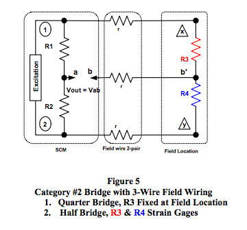
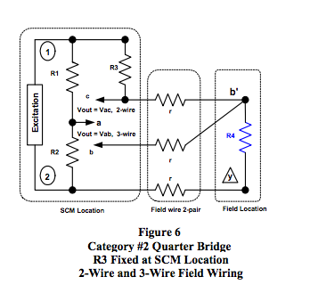
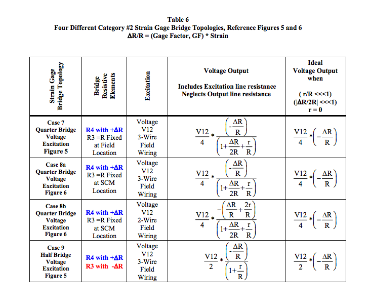
Table 6 in the Appendix illustrates output voltage expressions for four different implementation configurations of the bridge circuit shown in Figures 5 and 6 where the strain gage elements exposed to beam strain are located as shown in Figure 2. In all cases, the output voltage line resistance is ignored as justified in Reference 1.
- Quarter Bridge: Case 7 and Case 8
Bridge elements R1, R2, and R3 are fixed equal to R.
The strain gage element is R4 and is located as shown
in Figure 2.
Case 7, Figure 5: R3 is fixed =R and is field located using 3-wire field wiring.
Case 8a, Figure 6: R3 is fixed = R and is located at the SCM using 3-wire field wiring.
Case 8b, Figure 6: R3 is fixed = R and is located at the SCM using 2-wire field wiring.
- Half Bridge: Case 9 Bridge elements R1 and R2 are fixed equal to R. Strain gage elements R3 and R4 are located as shown in Figure 2.
Strain Gage Bridge Topology Conclusions
Upon examination of Figures 4, 5, and 6 with Appendix Tables 5 and 6, three salient observations are evident:- IF (2r/R << 1) AND IF (ΔR/R << 1), then the strain gage output voltage is directly proportional to ΔR/R independent of bridge circuit topology. Consequently, for strain gages ΔR/R = GF*strain, bridge output voltages are linearly proportional to strain within the above constraints.
- Excitation line resistance “r” has no effect in Category #1 full R-Bridge topologies with current excitation.
- Current excitation is not advisable for Category #2 quarter and half bridge topologies where the bridge elements R1 and R2 are contained within the SCM.
Beam Bending Measurement Example
Dataforth does not necessarily suggest that this method of measuring beam bending deflection, strain, and stress is optimum or particularly practical. This example is presented only as an illustration of interfacing strain gages to Dataforth SCMs and identifying the impact of associated errors.The 120 ohm foil strain gage specified in Table 2 is chosen for the active bridge element(s).
By choice, the SCM will be located 15 feet from the point of measurement (POM), which requires 20 feet of #20 AWG copper field wiring to connect the bridge circuit to the SCM. The DC resistance for 20 AWG copper wire is 10.4 ohms per 1000 feet. For this installation, a line resistance is r = 0.208 ohms, and r/R = 0.001733. The condition (2r/R << 1) is sufficiently true.
The strain gage elements will be located 2 inches from the left beam end, where the mathematical model of our beam example that is shown in Figures 2 and 3 predicts a strain of -1079μ in/in and the bottom surface of the beam is in tension. This strain yields Δ R/R = -0.00216; recall from Equation 6 that Δ R/R = GF*strain. It is important to observe here that the condition (|Δ R/R| << 1) is sufficiently true.
A Category #2 half bridge 3-wire strain gage bridge topology will be used with R3 and R4 located as shown in Figures 2 and 5. Appendix Table 6 Case 9 describes the output expression for this topology. As chosen for this example, Figure 7 illustrates Dataforth’s SCM5B38-03 with a 3.333VDC excitation source, 3mV/V sensitivity, a ±5 volt output, and a 10kHz bandwidth. Sensitivity is specified as the full-scale change in bridge output in millivolts per volt of excitation voltage provided. Considering the SCM as a voltage amplifier, the input range is determined by multiplying the sensitivity by the excitation voltage. 3mV/V * 3.333V = ±10mV. The resulting voltage transfer function, or gain, is ±5V/ ±10mV = 500V/V. Based on application, there are many other SCM5B38 models to choose from with different excitation voltages, sensitivities, output ranges, and filter bandwidths.
The exact error free SCM voltage output for this proposed measurement system on the beam with the strain gage located as shown in Figure 2 is -1.7975VDC.
Sources of Measurement Errors
Previous analytic expressions have assumed R-Bridge environments where all bridge resistive elements are equal in the absence of process variables. However, when one purchases individual bridge elements, they may not be matched. Equation 7 illustrates the voltage output for the above example of an SCM Category #2 half bridge 3- wire strain gage application where the active bridge elements are R3 and R4 as shown in Figures 2 and 5.SCM output voltage, Vout, is
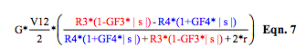
If strain gage elements are identical, Equation 7 becomes
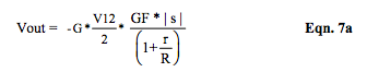
where G is SCM gain and V12 is the excitation voltage, GF3 and GF4 are R3 and R4 gage factors, s and s are the top and bottom beam bending strain magnitudes.
The signal conditioning module’s gain, excitation voltage, and internal errors contribute to measurement inaccuracy. Mismatches in strain gage elements and the associated mismatches in their bonding to the beam also are contributors to measurement errors. In addition, the effect of temperature on all system components adds errors. The following examination of errors assumes that the bonding is such that top and bottom beam surface gage bending strain magnitudes are identical.
Output Line Resistance Error
The extremely high input resistance of Dataforth’s SCMs allows us to neglect the voltage divider effect of output voltage line resistance; see Reference 1.
Excitation Line Resistance Error The equations in Appendix Tables 5 and 6 clearly show two situations where excitation line resistance can be eliminated or neglected.
- Current excitation for Category #1 full R-bridges will completely eliminate excitation line resistance.
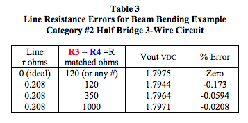
- In Category #2 bridge configurations, excitation line resistance can be neglected if 2r/R is <<1. Note that larger “R” values for strain gage elements help minimize the effects of excitation line resistance. Table 3 illustrates this.
Resistive Bridge Element Mismatch Error
Strain gage bridge circuits are sensitive to small changes in resistance and operate within a small region around bridge balance. This requires strain gage elements to be identical (i.e., equal gage factors and equal resistors in the absence of process variables). Recall that identical strain gage elements were assumed in the previous expressions.
Table 4 shows the effect of non-identical strain gages for the above beam bending example. Strain gage mismatches cause a nonzero output, Voff, in the absence of process variables. The output voltage, Vout, is incorrect but can be corrected by subtracting Voff. Table 4 values are rounded.
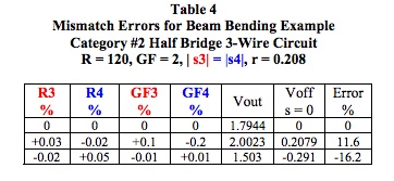
It is important to observe that small mismatches in strain gage elements can cause significant system measurement errors. Most strain gage manufacturers provide strain gages packaged in groups that are all from the same manufacturing lot; therefore, these units are reasonably well matched. In addition, the resistance and gage factor values are identified on each unit. Nonetheless, mismatches may occur. Strain gage manufacturers have excellent technical support and should always be consulted regarding applications using their products.
Corrections for mismatches and calibrations can be performed within the user’s data acquisition software program or by using SCMs with “Zero and Span Adjust” functionality. Dataforth offers a complete bridge strain gage SCM DIN rail product line, DSCA38, with zero and span adjustment functionality; see Reference 4.
Signal Conditioning Module Error
Dataforth’s strain gage bridge modules have a ±0.03% accuracy specification with a ±0.03% specification on the isolated field voltage available for bridge excitation. Per previous discussions, Tables 3 and 4 illustrate that errors due to line resistance and mismatches in bridge elements are typically responsible for the major portion of measurement errors. Observation of these resulting errors illustrates that Dataforth’s SCM is an insignificant source of measurement error.
Dataforth SCM Protection
Each different strain gage bridge measurement topology has associated inaccuracies. Other undesirable error hazards such as electrostatic discharge (ESD) transients, common-mode voltages, ground loop currents, etc., exist between the test unit location and instrument equipment. These hazards must be minimized for enhanced overall accuracy. Dataforth’s signal conditioning modules provide levels of hazard protection not available in most competitive brands.Dataforth SCMs provide transient protection, overload protection, and 4-way isolation. Four-way isolation provides isolated excitation power to the bridge, isolated power to the field-side electronics, isolated power for system-side electronics, and an isolated signal path to the instrumentation device. Dataforth SCMs’ protection features essentially remove ground-loop problems and minimize both electrostatic discharge damage and damage due to excessive common-mode voltage. Wiring protection against wiring errors is included as well. Dataforth’s transient protection exceeds the ANSI/IEEE C37.90.1 specification. Moreover, input and excitation connections are all protected to 240VAC continuous.
Dataforth References
- Dataforth Corp., AN117
http://liwww.dataforth.com - Dataforth Corp., AN105
http://liwww.dataforth.com - Mechanics of Materials 2e by F.P. Beer and E. R. Johnson McGraw Hill
- Dataforth Corp.
http://liwww.dataforth.com
APPENDIX
This appendix contains Schematics of Dataforth Bridge SCM5B38-03 and Tables of Output Voltage Expressions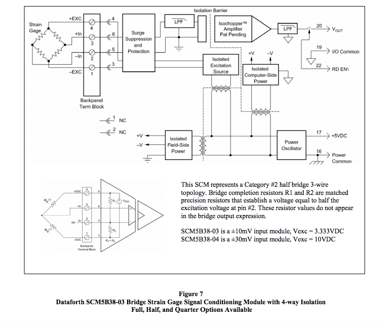
Was this content helpful?
Thank you for your feedback!