RMS Revisited (AN128)

Preamble

When we purchase electrical equipment, appliances, light bulbs, motors, heaters and such, somewhere on the “name plate” are some electrical specifications such as voltage, current, frequency, power, etc. We have seen these values for as long as we have been able to read and so we just take them for granted. For AC (the abbreviation for alternating current), the values for voltage and current are always shown as “RMS” values; however, this fact is rarely stated on the name plate. It is assumed everyone knows this.

What does RMS really mean? This Application Note will revisit the definition of RMS, show RMS values for various time functions, and explore some interesting RMS measurement issues. Our object here is to provide a better understanding of some of the subtle characteristics of RMS. However, reviewing RMS values for time functions containing random components is beyond the scope of this Application Note.

The Appendix contains additional information for your reference, and the reader is encouraged to examine the previous Dataforth Application Note on RMS, AN101.

RMS Definition Revisited

Throughout this Application Note, we will consider only periodic functions with no random components. The way to think of the RMS value for a time varying function of voltage or current is to recognize that an RMS value for these time varying items means that the time varying function has the same energy capacity as some value of DC (abbreviation for direct current) voltage or current.

The derivation of RMS begins with the requirement that the function of time is “well” behaved (bounded with a finite number of discontinuities), repetitive at some fundamental frequency, and available for as long as needed. A pure mathematician might cringe at these simple requirements but we engineers love them because they apply to most types of voltages and currents we deal with in practice.

The experimental apparatus is a pure resistive heating element within a perfectly thermally insulated container. An ideal DC voltage (say 10 volts) is connected to this heater until thermal equilibrium is reached with a final temperature of say Tx degrees.

Next, this DC voltage is removed, the unit is allowed to cool down, and a time varying voltage, V(t), is applied to the heater until thermal equilibrium is again reached with a final temperature of, say, Ty degrees. If Ty = Tx, then the effective value of V(t) = 10 volts (same as the previous DC value) and so we say the RMS value of V(t) is effectively 10 DC volts. Why the name RMS? The name comes from the mathematics of this experiment as follows:



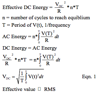
A careful look at this mathematical equation shows that it is the Root of the Mean (average) value of V(t) Squared. Hence, the name RMS.

RMS Examples

Perhaps the most familiar time function is the sinusoidal function. Recall that a sinusoidal function can be described as a sine function or cosine function depending on where we choose to place the time origin. As you know, the utility companies go to great lengths to ensure the voltage on their power grid distribution system is a sinusoidal voltage function. Consequently, the RMS value of sinusoidal functions of time is the dominant focus in most introductory electric circuit courses and little time is spent on determining RMS values for unusual shaped functions of time.

Most of us recall the RMS of a sinusoidal function as:



For example, consider the name plate specifications of a toaster showing 120VAC, 60Hz. This means the actual utility line voltage out of the wall socket is a 60Hz sinusoidal voltage function with a peak value of 169.7 volts. This utility supply voltage function of time is commonly expressed by either of the following sinusoids:

v(t) = 169.7*Sin(2*π*60*t)
v(t) = 169.7*Cos(2*π*60*t)

All this is well and good but the fact is there are scores of other functions of time that we need to measure that are nowhere near sinusoidal. So what about these? As an example, consider nonlinear loads on the utility’s fixed sinusoidal voltage line; the load currents will in no way be sinusoidal but we need to measure them nonetheless.



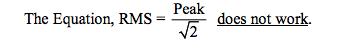
Table 1 (page 7) illustrates some common nonsinusoidal time functions and their associated RMS values. Take a look, you may be surprised.

Parceval’s Theorem

Parceval’s Theorem is a handy trick to know. As an illustrative example of using this theorem, consider the situation where an auxiliary emergency backup generator is connected to a facility. It is possible for such generators to create sinusoidal harmonics on the customer’s supply lines. Sometimes such generator’s specifications give the harmonic content. Figure 1 illustrates a situation where the composite voltage is a sum of four different RMS voltages, one at a fundamental frequency, one at the third harmonic, one at the fifth harmonic, and a DC average.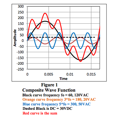



So what is the RMS value of the RED function of time? Do you want to write an equation for it and use Eqn. 1? Well, we could but it would be messy so instead let us use Parceval’s Theorem, which says that for a composite function composed of different functions, the RMS value can be calculated by the following:



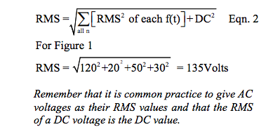
We will show more practical examples of Parceval’s Theorem later on when we use the Fourier Series to calculate RMS.

Measuring RMS

Any module that measures the RMS value of a time varying function must, in general, implement Eqn. 1 (page 2). The modern techniques and circuit topologies of such devices are far beyond the scope of this Application Note. Moreover, most vendors of such devices consider their methods to be intellectual property (IP) and do not publicize their circuits and embedded software (if any). Companies that supply RMS modules use various implementations of Eqn. 1 ranging from simple analogy circuit topologies to sophisticated digital sampling with Digital Signal Processing (DSP) microprocessors running special software algorithms. However, as a selection aid, device specifications are always provided.

For example, Dataforth RMS Measurement Modules provide specifications that include:

1. Component Drift
2. Component Aging
3. Temperature Variation
4. Supply Voltage Variation
5. Humidity
6. Circuit Linearity
7. Circuit Repeatability and Hysteresis
8. Common Mode Voltage Rejection
9. Transient Protection
10. Frequency Response
11. Crest Form Factor

Most readers are familiar with the analog specifications 1-9 and how they apply to their specific requirements; therefore, we will not dwell on these in this Application Note. However, Frequency Response and Crest Factor (Form Factor) specifications may need a little additional examination.

Non-Sinusoidal Measurement Example

As a typical example of a non-sinusoidal time function, consider the situation in which a 60Hz utility supply is connected to a non-linear load. We will use for illustration purposes a full wave bridge rectifier as the non-linear load. Industrial facilities have speed drive for induction motors, controllers for DC motors, welders, and large dimmer units. In general, all these have within their circuit topology some form of AC to DC converter and may or may not have an input line filter.

Figure 2 shows the typical wave forms in this situation.



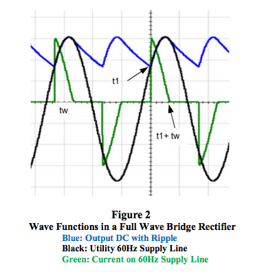
Notice that the output is a DC voltage with a rippling value at 120Hz riding on top of an average (DC) value. Perhaps most surprising is the green line current pulse shaped like a sawtooth with a frequency at twice the line frequency, 120Hz. So what is the RMS value of this current pulse?

The Fourier Series
Recall Fourier’s theorem, which says that a function of time “f(t)” can be expressed as a sum of sine and cosine functions over an infinite number of frequencies plus an average value term. At this point, a mathematician would hasten to give us all the limitations for this theorem; however, most engineering voltages and currents we work with are “well” behaved and Fourier’s theorem applies. The following form of this theorem will allow us to demonstrate the effects of frequency on RMS measurements.



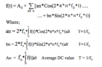
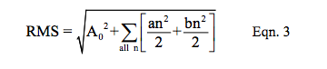
Note that “f₀” is the signal “f(t)” frequency and that “an” is the peak amplitude of the “n^th” Cosine harmonic and “bn” is the peak coefficient of the “n^th” Sine harmonic. Remember that a non-sinusoidal time function contains many (infinite number in theory) different frequency harmonics. We can use this fact to calculate the RMS of non-sinusoidal time functions by using Parceval’s Theorem for RMS, which is:



Recall, RMS is Vpeak ÷ square root 2.

We hasten to point out that all this is interesting; however, the shape of a time function whose RMS value we wish to measure is seldom, if ever, known. So what is the value of this nasty math? From a practical point of view we rarely use this analysis to actually calculate RMS since the equation for the quantity we wish to measure is unknown. However, we are going to use this analysis in examples to illustrate the frequency requirements of measuring non-sinusoidal functions and therein lies the value of this nasty math.

Example 1
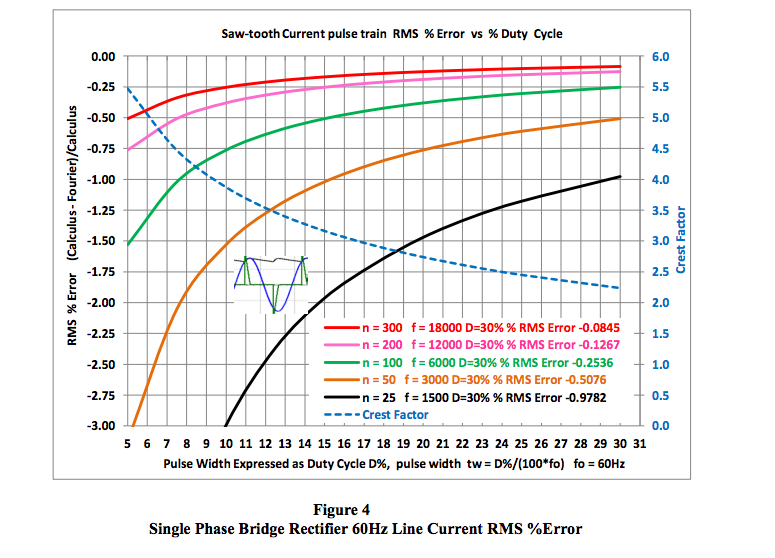
Figure 2 (page 4) shows the actual 60Hz line current in typical industrial equipment containing bridge rectifiers. This green line current approximates a sawtooth wave form.

To partially simplify the mathematical calculations, we will model this sawtooth function as:



The pulse shape and specifically the pulse width “t_w” is determined by the load resistance, the filter capacitance, and the supply frequency. Figure 8 (Appendix 2, page 13) shows an example of how pulse widths can vary with load resistance for several given filter capacitances. The model used here (shown above) is sufficiently accurate to illustrate our objective, which is to show the effects of frequency content in this common type non-sinusoidal line current. Remember that “f₀” is the driving source frequency (60Hz in this example) not the pulse frequency.

Reexamine the bipolar sawtooth line current function shown as green in Figure 2. The graph in Figure 4 (page 8) illustrates how RMS %Error as a function of base line pulse width expressed as Duty cycle varies with different “n” numbers, i.e. frequency components.

Note Results in Figure 4
1. For any given number of frequency harmonics (n value) the RMS %Error decreases as %D increases, that is as t_w increases RMS %Error decreases for any given n.
2. For any pulse width t_w given as %D, the RMS %Error decreases as number of frequency harmonics (n) increases.

The nasty math in this example shows the 60Hz line current RMS %Error for 30 %D and 300 frequency components is -0.0845%. However, to achieve this accuracy (at 30 %D and n = 300) requires the measurement device to have a frequency response in excess of 18,000Hz (60*300).

Example 2
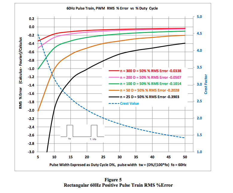
The second entry #2 of Table 1 (page 7) illustrates a Positive Pulse Train with a fixed frequency and varying base line pulse width. This sort of time function is analogous to a pulse width modulation (PWM) device used in such applications as load dimmers, and speed controllers, etc. Although such devices are more complex than this simple example, it is adequate to illustrate our objective, which is to show another example of how RMS values are dependent on pulse width and frequency content. The results of this analysis are very similar to the analysis in Example 1. Examine Figure 5 (page 9) and notice again how RMS value depends on the frequency content of the measured pulse train.

Example 3
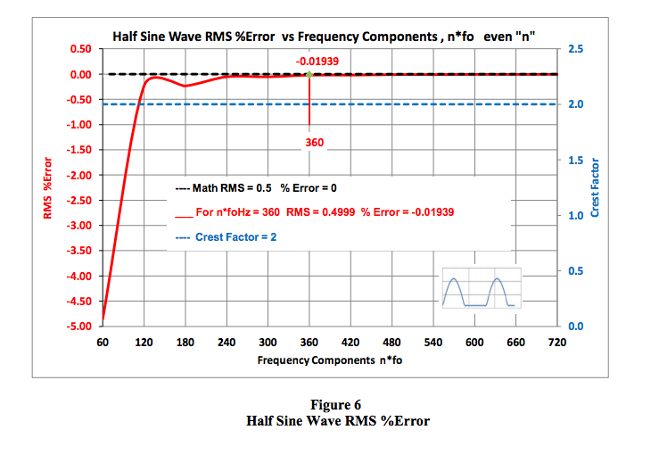
Consider a half-wave rectified sine wave as shown in blue for the #6 entry of Table 1 (page 7). It is clear that the time function is just the positive half of a sine wave at some frequency, “f₀”. In addition we see that this function does not have sharp corners with varying base line widths; therefore, we intuitively suspect that the frequency content (harmonics of f₀) will be small. Figure 6 (page10) clearly illustrates this. Similar results apply to the Full Wave Rectified Sine Wave, entry #7 in Table 1.

Another Surprise Example
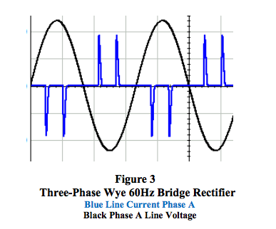
Consider the case where a 50 horsepower DC motor is driven by a 60Hz three-phase balanced Wye AC to DC speed controller containing a non-line filtered bridge rectifier. We want to measure the RMS phase line current in one 60Hz phase voltage line.

Figure 3 for this proposed situation shows in blue the three-phase line current in phase A. Is this a surprise? Can your RMS measurement device correctly measure RMS values of this type 60Hz line current?

Equations

Appendix 1 (page 12) displays Fourier Series equations for examples used in this Application Note.

Crest Factor

Another interesting specification on RMS measurement modules is the Crest Factor, sometimes called the Form Factor. Error due to Crest Factor is an often stated specification for RMS measurement devices. Crest Factor is defined as: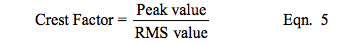



Using the Crest Factor specification as a selection guide requires that one knows both the peak amplitude value and the RMS value of the time function to be measured. Unfortunately both are unknown before measurements are made. Therefore, it is essentially impossible to specify an RMS error associated with the Crest Factor for all possible non-sinusoidal time functions. Nevertheless, RMS measurement module suppliers do show a range of Crest Factor errors that a buyer can use to get a “handle” on possible RMS errors caused by non-sinusoidal shaped time function for a given RMS measurement application.

The Conclusion

The above examples illustrate that when measuring RMS one should try to determine what is being measured and make sure the RMS measurement device has adequate frequency response, in excess of n*f₀. This may be somewhat difficult to do accurately since one does not usually know beforehand the shape of the signal to be measured and exactly how many (“n”) harmonic frequencies are necessary to achieve a required accuracy in the RMS measurement.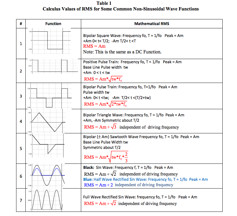



The graph shown below in Figure 4 is a sample illustration of how the RMS error value of a sawtooth bipolar pulse varies with base line pulse width (t_w) expressed in % Duty Cycle and number (n) of harmonic frequency components. In addition, the variation in Crest Factor is shown.



The graph shown below in Figure 5 is another sample illustration of how the RMS error value of a non-sinusoidal rectangular positive pulse train wave form varies with base line pulse width (t_w) expressed in % Duty Cycle and number (n) of harmonic frequency components. Pulse trains of this nature are analogous to pulse width modulation, PWM devices. In addition, the variation in Crest Factor is shown.



The graph shown below in Figure 6 is a special example of how the half wave rectified Sine wave RMS error value varies with the number (n) of harmonic frequency components. As shown, a relatively small number of harmonic frequency components (three in this graph) is required to establish a tiny RMS %Error. This is expected, since the pulse width is exactly half a period and the function is a smooth completely defined sinusoid. In addition, the Crest Factor is shown as a constant value of two.



DATAFORTH RMS MEASUREMENT DEVICES
True RMS measurements require instrumentation devices that accurately implement the RMS equation. Dataforth has developed three RMS module families that do just that: the SCM5B33, SensorLex® 8B33, and DSCA33. All three families are made up of isolated True RMS input modules that provide 1500Vrms transformer isolation. Each module provides a single channel of AC input that is converted to its True RMS DC value, filtered, isolated, amplified, and converted to standard process voltage or current output (Figure 7 below). The SCM5B33 and SensorLex 8B33 are plug-in-panel products; the DSCA33 is a DIN rail mount device.



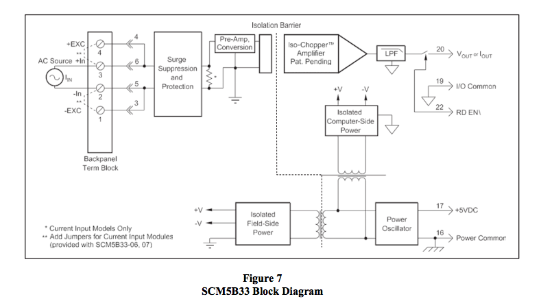
Block diagrams for the 8B33 and DSCA33 are very similar to the 5B33.

References:

1. Dataforth Corp., http://liwww.dataforth.com
2. Dataforth AN101 Measuring RMS Values of Voltage and Current,
   http://liwww.dataforth.com/catalog/pdf/an101.pdf

Appendix

Appendix.1
Fourier Series equations for examples in this Application Note are shown below for your reference. Recall for all time periodic well behaved functions “f(t)” the Fourier Series representation is:

• f(t) = ao + n over all “n” for [ an*Cos(n*2*π*fo*t) + bn*Sin(n*2*π*fo*t]
• “n” is the number of a particular frequency harmonic, n = 1 to infinity is the limit
• “fo” is driving source frequency, T = 1/fo
  
• Fourier RMS = {ao^2 + n over all “n” for [(an^2 + bn^2)/2]}^0.5
• Calculus Crest Value = Am ÷ RMS Value Where Am is Amplitude maximum = Vpeak

1a. Bipolar Square Wave, #1 in Table 1

2a. Positive Pulse Train, #2 in Table 1

3a. Bipolar Pulse Train, #3 in Table 1
4a. Triangle Wave, #4 in Table1
5a. Bipolar Sawtooth Wave, #5 in Table 1
6a. Half Wave Rectified Sin Wave, #6 in Table 1
7a. Full Wave Rectified Sin Wave, #7 in Table 1

Appendix 2.
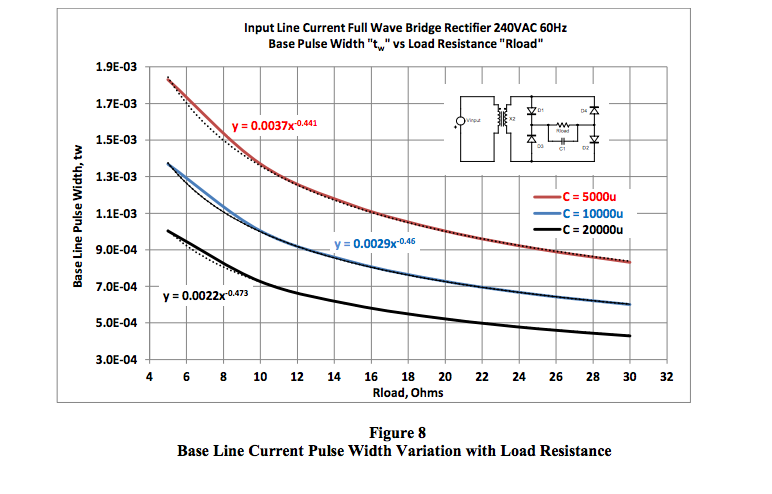
Some interesting results are shown below in Figure 8. Given our ideal model (Equation 4) of a sawtooth line current pulse train, the empirical data shown in Figure 8 illustrates the variation trend in base line pulse width (t_w) with load resistance for various values of filter capacitance.



Appendix 3.
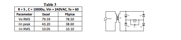
Table 3 shown below illustrates a comparison between the assumed ideal model of a current sawtooth pulse used in this Application Note to analyze a full wave bridge rectifier and a PSpice simulation of an actual bridge full wave rectifier. Although the individual results are not identical, the comparisons are close enough to justify the ideal model used for our Fourier Series analysis. Remember that PSpice simulation uses real models for circuit elements whereas our model uses ideal components.



Appendix 4.
The output of a full wave rectifier with a capacitor filter has both a DC value and a ripple component determined by the input AC RMS voltage, input driving frequency, and the rectifier circuit components such as filter capacitance and load resistor. See Figure 2 (page 4) for a reference.

Using Parceval’s Theorem we could determine the output RMS value. Unfortunately, we do not know beforehand the individual RMS values of the DC and Ripple component. You may find interesting the equations shown below, which represent an analytic effort to calculate the output RMS voltage and the peak current occurring at the instant the filter capacitor begins to charge. The following equations are derived using our Excel model, (Equation 4 page 5). Table 3 above illustrates the comparison results.

4a. VoRMS = [(Vin*2^0.5)*((Rload*C*fo*(1-EXP(-2*t1/(Rload*C)) + 0.5
4b. Ipeak = ((VinRMS/X2)*2^0.5)*(C*2*π*fo)*Sin(2*π*fo*t1) + (-VinRMS/X2)*2^0.5)*Cos(2*π*fo*t1))/(Rload*X2)

Where:(a) X2 is Transformer turns ratio (X2 in all above examples is 4:1, 1/X2 = 0.25 (b) t1 is exponential decay time of filter capacitance and is equal to solution of EXP(-t1/(Rload*C)) + Cos(2*π*fo*t1) = 0 One can solve using: HP49g+ calculator, Mathcad, MatLab, Excel Solver, etc. (c) t_w = 1/(2*fo) - t1

4c. i(t)RMS = Ipeak*(fo* t_w*2/3)^0.5 For i(t) = ipeak*(1-t/t_w)