


an109: Single Phase AC Measurements Revisited
Application Note
Preamble
Alternating Current (AC) systems are analyzed using "phasor algebra" ala Stienmetz. Most engineering students initially learn this technique as it applies to single-phase systems. These training exercises often included multiple voltage sources with arbitrary phase angles (voltage phasors) as practice in phasor manipulations. Such exercises were generally more focused toward training in phasor manipulations than modeling real electrical systems.The objective of this brief application note is a simplified review of practical single-phase current calculations using phasors and "name-plate" data. A similar review of three-phase calculations is available in Dataforth’s Application Note AN110, Reference 1.
Real-time AC current and voltage calculations, prior to measurements, can be very helpful in the selection of signal conditioning modules. Dataforth offers excellent high-voltage attenuation products to safely divide-down, isolate, and condition potentially dangerous single-phase AC potentials. See Dataforth’s SCMVAS product family, Reference 4.
Years ago, in the late 1800 hundreds, Thomas Edison’s DC approach to power transmission lost the race to George Westinghouse’s AC approach to power transmission. Consequently, today’s industrial, commercial, and residential voltage distribution systems use AC sinusoidal voltages to supply electrical energy.
Ohm and Kirchhoff develo ped the basic concepts of DC circuit analysis over 200 years ago. Applications of these concepts to real-time manual analysis of AC sinusoidal circuits is extremely difficult because in DC systems, current and voltage are always in phase; whereas, AC currents and voltages are not necessarily in phase when periodic time varying (AC) sources are involved.
Quick Review of Conventions and Definitions
All utility companies use synchronous generators in their generating plants. These machines produce sinusoidal voltages with the waveform shown in Figure 1.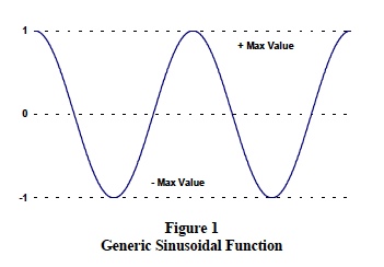
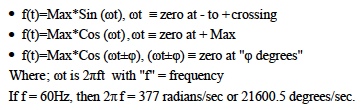
Sinusoidal waveforms have several mathematical representations, for example;
Each of these representations correctly describes sinusoidal functionality as shown in Figure 1. The important distinction between these representations is where "zero time" reference is arbitrarily chosen.
Phasors
Consider a line of length "Max" initially at rest on the x-axis. If this line rotates in a counterclockwise direction at an angular rate of 60 revolutions per second, the projection (shadow) of this rotating line on the x-axis oscillates back and forth with "cosine functionality". This shows that; Real-time cosine functionality can be represented by the projection ("shadow") of a counterclockwise rotating vector on the x-axis (labeled "real-axis"). This defines a "phasor" and establishes the popular convention of representing real-time sinusoidal voltages/currents with "phasor" cosine functionality. For brevity, Steinmetz’s proof is omitted..Equation 1 shows the phasor representation of a 120-volt (rms) voltage source with a cosine time expression. Equation 2 shows the same voltage function with a lagging phase angle of 60 degrees. For a review on RMS values, see Dataforth’s Application Note AN101, Reference 2. In addition, examine Reference 5 to see Dataforth’s product line of signal-conditioning modules for converting AC inputs to True RMS voltages.
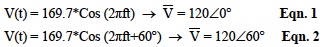
Note: This phasor notation allows using vector math for analyzing sinusoidal voltages and currents.
Ohmic Behavior of Inductance and Capacitance
Current and voltage relationships associated with inductors and capacitance are dependent upon rates of change with respect to time. Voltage rates of change determine inductor currents; whereas, current rates of change determine capacitor voltages. Equations 3 and 4 describe mathematical models for this natural behavior.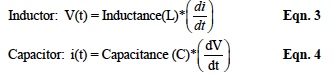
If 120-volt RMS cosine functions {120*cos(ωt)} are substituted Equation 3, and 4, mathematical manipulations give the results shown in Equation 5, 5a ,6,and 6a.
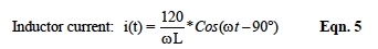
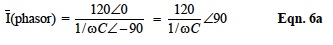
Equation 5 illustrates that inductor current is the inductor voltage divided by the Ohmic term (ωL) and LAGS the voltage by 90 degrees. Manipulating Equation 5 with gives;
In like manner, the current in a capacitance is determined as shown in Equation 6.
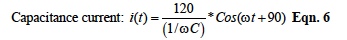
Equation 6 shows that capacitor current is the capacitor voltage divided by the Ohmic term (1/ωC) and LEADS the voltage by 90 degrees. Manipulating Equation 6 gives;
AC Impedance
Equations 5a and 6a are analogous to Ohm’s Law for DC circuits. These equations show a similar relationship; namely, that an AC current phasor is equal to a phasor voltage divided by an Ohmic term. This "AC resistance" is defined as "reactance" with the symbol "X". For inductors, XL is ωL Ohms; for capacitance, XC is 1/ωC Ohms. In addition, to this Ohmic behavior, there is an accompanying 90-degree phase shift between current and voltage under sinusoidal excitation.Charles P. Steinmetz mathematically modeled this behavior with "complex number" algebra. Pure resistance (R) is placed on the x-axis, labeled "real" axis. Inductive reactance (XL) is located on the positive y-axis, labeled positive imaginary axis with symbol "+j". Capacitive reactance (XC) is located on the negative y-axis, labeled negative imaginary axis with symbol "-j". There is nothing imaginary about these axes; they are just orthogonal to the horizontal "real" axis. However, a hundred years of history and thousands of textbooks have used "imaginary" to indicate electrical quantities with a phase angle of ± 90 degrees are located on the ± j-axis.
For example, Steinmetz’s mathematically model of a pure three Ohm inductive impedance is the complex number vector, Z = ( 0+ j3).
Figure 2 shows R, L, and C elements connected in different arrangements, each of which develop different AC impedances (Z12) between points 1 and 2.
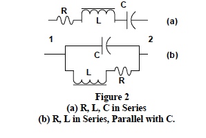
Combining series elements and parallel elements the two expressions for impedance Z12 in Figure 2 are;
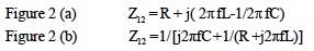
Both these equations can be arranged into the same complex number vector format as shown below;

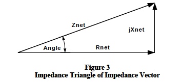
Regardless of the circuit topology, any ensemble of R’s, L’s, and C’s can be reduced to a simple complex impedance number, which can be illustrated by an impedance triangle as shown in Figure 3.
AC Power
The impedance triangle shown in Figure 3 represents a composite series impedance and can be scaled by multiplying each side by the current, creating a net "voltage" triangle; scaling again by multiplying each side by the current creates the "Power Triangle" shown in Figure 4.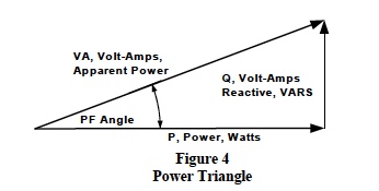
Power is the time rate of energy transfer (utilization) averaged over one sinusoidal cycle with the units of “energy” per second. Electrical power has the units of “watts” and can be expressed as; joules per second, foot-pounds per second (horsepower), BTU’s per hour etc. In electrical systems, watts (joules/sec) is determined by the product,” volts*amperes”. In DC circuits, volts and amperes are in phase (no phase shifts in DC systems) and V*I is a real number on the x-axis representing “real” power. One should think of “real” power as the time rate of change of the energy associated with doing useful work. The situation is a bit more complicated in AC systems.
Figure 4 illustrates that there are three quantities, which can be represented by the product V*I. All three of these V*I quantities have the units of joules per second (watts), but each represents different characteristics. The product of applied voltage and the associated input current has units of watts and “appears” to be “the” power. However, Figure 4 shows, that this product is a vector represented by the complex number (P + jQ). Power (P) on the real x-axis represents the component of V*I that is responsible for doing real work. Reactive volt-amps (Q) on the j-axis represents the component of V*I that is associated with the system’s reactive elements (inductance/capacitance) and does no useful work. Basic relationships of the power triangle are;
- Apparent Power is V*I, units of Volt-Amps-Apparent
- Power Factor (PF) is Cosine of angle that current leads/lags voltage, no unites
- Real Power (P) is V*I*Cosine of PF Angle, units watts, P=V*I*(PF) or P= I2*Rnet
- Reactive Power (Q) is V*I*Sine of PF Angle, units of VARS (Volt-Amps-Reactive)
Note: Inductive loads cause lagging power factors but are represented as positive jQ on the power triangle. Capacitive loads cause leading power factors but are represented as negative jQ on the power triangle
An analysis of the instantaneous time-domain product of V*I for each impedance element in an AC system shows;
- the instantaneous product of V*I across any element is a sinusoidal time function with a repetition rate of twice the frequency (2f) of the voltage and current,
- the instantaneous product of V*I associated with Rnet is “real” power (P) and has an average value of I2*Rnet or V*I*(PF) , and
- the instantaneous product of V*I associated with Xnet is the “reactive power” (Q) and is a symmetrical sinusoidal with an average value of zero. This reactive power (Q) does no useful work. In fact, this power “flows” back and forth between the utility company and the customer twice in each voltage cycle and creates heat losses in the distribution system.
Sample Calculations
Manufacturers do not generally give specific values for R, L, and C associated with their products. Nonetheless, the total AC system operating status (current, power, and PF) can be calculated from the manufacturer’s “nameplate” data. The following examples illustrate how these calculations are implemented.Calculations on AC Systems containing multiple loads with different phase angles are fundamentally straightforward but often are messy and confusing. The following list offers some helpful calculation “rules”.
- Choose one and only one voltage to be the phasor reference for all calculations. Maintain this reference at all times for all calculations.
- Use only RMS values. This avoids confusing sinusoidal peaks with RMS.
- Assume all line currents (L1, L2, and L3) flow into loads and all neutral (white wire) currents flow back (return) toward the supply source.
- Keep in mind that inductor currents lag the associated inductor voltage; whereas, capacitor currents lead the associated capacitor voltage.
- Determine the voltage and current directional subscripts and maintain strict adherence to the order of these subscripts; For example V34 means the voltage is a drop from point 3 to point 4; “3” is more positive than “4”. Note that; Vab = -Vba and Iab = -Iba.
- Voltage across any load follows the Ohm’s law convention, which states that the voltage drop (plus to minus in the direction of current flow) across an impedance is equal to that impedance multiplied by the current flowing (plus to minus) through the impedance; V12 (drop) = Z*I12.
- When drawing a phasor vector, the arrowhead is plus and the vector tail is minus; Vab is (b) --> (a).
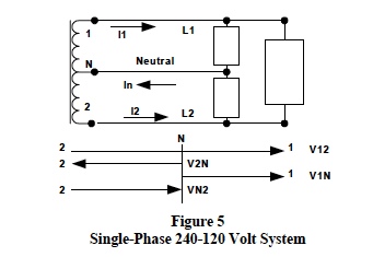
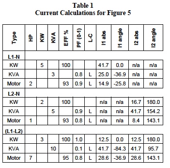
Figure 5 represents a standard single-phase 240-120 volt distribution system. This type system has three areas of loads; 240-volt (L1-L2) loads, 120-volt (L1-N) loads, and 120-volt (L2-N) loads. Most load situations can be modeled with the three types of load categories shown in the following list. In this list “Vline” is defined as the voltage across the given load.
- Motor loads with horsepower (HP), efficiency (EFF) and power factor (PF) data given. Single-phase line current equals [HP*746/(EFF*PF)]/Vline at an angle whose trigonometric cosine is equal to the power factor, lagging or leading the applied voltage.
- KW loads with the efficiency (EFF) data optional. Single-phase line current is [KW/EFF]/Vline at an angle of zero, PF =1.
- KVA loads with efficiency (EFF) and power factor (PF) data given. Single-phase line current equals [KVA/(EFF*PF)]/Vline at an angle whose cosine is equal the power factor, lagging or leading the applied voltage.
Table 1 shows the results of current calculations for arbitrary loads in Figure 5. Phasor reference is V12 at angle zero.
Notes:
- Loads between L1-L2 have no neutral current. Since V12 is reference, I1 flows into load, and I2 flows out; therefore in Figure 5, I2 = -I1.
- Calculations for loads between L2-N use VN2, which is – V2N (1/2 of V12, angle 180); therefore, I2 is in opposite direction as shown in Figure 5.
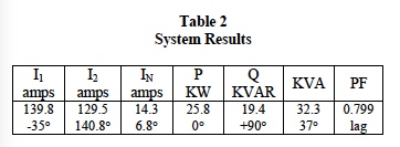
Detail calculations for the values in Tables 1 and 2 have been omitted for brevity; however, they follow the guidelines previously discussed. Readers are encouraged to validate these results.
The enthusiastic reader is invited to download Dataforth’s “Excel Interactive Work Book for Single Phase AC Calculations”, Reference 3. This file allows an investigator to simply enter nameplate data for all the system loads. Whereupon, this Excel interactive file automatically determines all line current phasors and the “power profile” quantities of P, Q, and PF. The effect of load changes can be instantly determined with this interactive file.
Dataforth References
- Application Note AN110: 3-Phase AC Calculations
- Application Note AN101: Measuring RMS Values of Voltage and Current
- Excel Interactive Work Book for Single Phase AC Calculations
- SCMVAS Voltage Attenuator System
- SCM5B33 Series of Modular True RMS Signal Conditioners
- Series of DIN Mount True RMS Signal Conditioners
Was this content helpful?
Thank you for your feedback!