Active, Analog, Elliptic Filter

History

Wilhelm Cauer, 1900-1945, is given credit for being the major, early contributor to the topic of electrical network synthesis. Prior to network synthesis, passive filters were designed by the image impedance method. Cauer’s work provided an exact solution including impedance matching at the termination.

He finished his doctorate and professorship requirements in Germany. Due to economic conditions in the 1930’s, he moved with his family to the United States where he worked at MIT and Harvard. There he worked with Vannevar Bush on analog computers to solve mathematical problems.

Wilhelm Cauer also had good relations with researchers at AT&T Bell Laboratories. His interest was to solve linear systems related to electronic filters. He returned to Germany with the intent of building a fast analog computer, but was unable to secure funding. There he worked in industry and lectured at the Technical University in Berlin.

Near the end of WWII and the expected fall of Berlin, he moved his family to the small town of Witzenhausen in Hesse, Germany. Against advice, he returned to Berlin and was executed by Russian soldiers.

Design

Elliptic filters, sometimes called Cauer filters, differ from Bessel, Butterworth, and Chebyshev filters in that they provide an equal ripple stopband as well as an equal ripple passband. They do this by having jω axis zeros. They may be designed to have a very abrupt transition from the pass band to the stop band.

For active circuits, one of the preferred ways to implement these filters is by using the State-Variable circuit (1). This is sometimes referred to as a KLN circuit after the authors of reference (1). With this circuit topology and a table, or source, of pole and zero positions, an elliptic filter may be readily realized.

For these positions, various sources are available. One is table 2.4-1, page 65 of the second reference (2). Another is tables 8.7 and 8.8, pages 8-10 and 8-11 of reference (3).

An even more versatile method is the free download, computer application FilterCAD. An internet search readily reveals several sources.

This application was first offered by Linear Technology, now acquired by Analog Devices Inc. The following implementation follows an elegant solution in Huelsman (2).

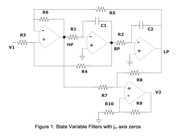
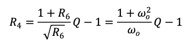
The circuit of figure 1 has three amplifiers with intermediate outputs labeled HP, BP, and LP for high, band, and lowpass. These first three amplifiers constitute the state-variable circuit. The fourth amplifier implements the elliptic filter function between V1 and V2. The first three equations recognize the general forms of the three intermediate outputs plus the fourth, V2 output formed by the addition of the high-pass and low-pass outputs.

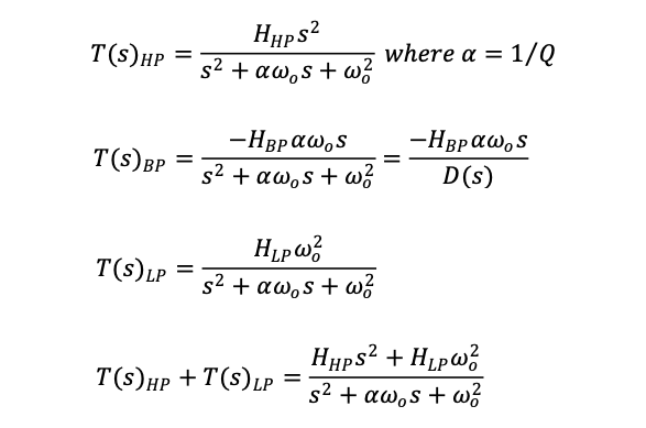
With this last equation, we clearly have what we need, a complex pole pair in the denominator and a jω axis zero pair in the numerator.

With the requisite node analysis and algebraic manipulations, we will find,

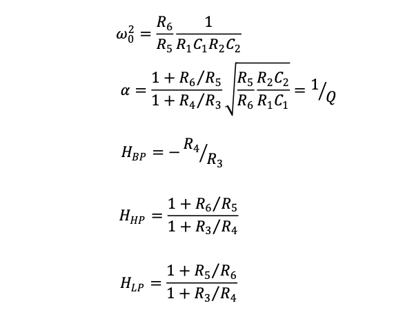
With further analysis and algebraic manipulation, the final transfer function is found to be,

Solving for R₄,

The DC gain of the transfer function is,

Solving this for R₁₀,

Given inputs for ω_z, ω_o, Q, G we have four simple formulas for R₄, R₆, R₇, R₁₀.

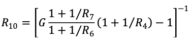
Usually, G = 2 is a good choice. For some low Q cases, G = 1 will work; otherwise, if G is too low, R₁₀ will be negative.

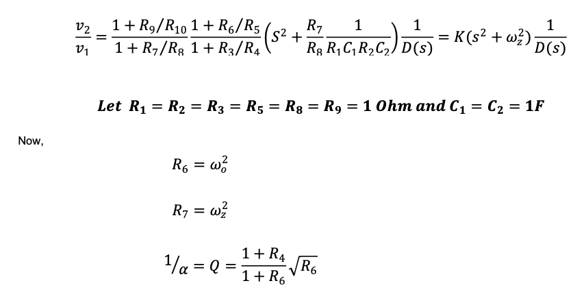
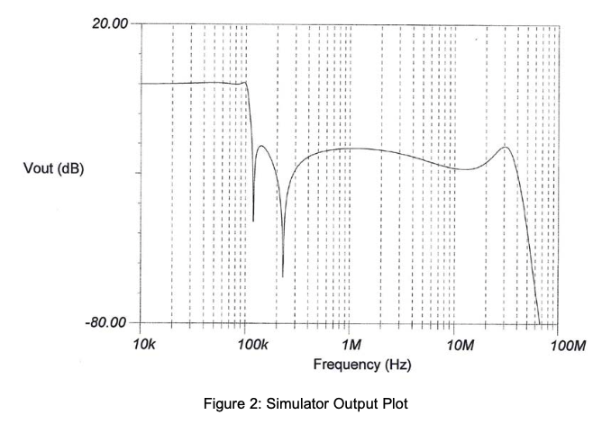
To verify that the final design equations work properly, a two-stage simulation was run on the Tina simulator. A gain of 2 was used to calculate R₁₀. The output plot is shown below. Note the two notch frequencies. For an overall gain of 1, a 2 to 1 attenuator was added to each stage by converting R₃ to the Thevenin equivalent, 2 to 1 attenuator circuit. The peaking at 30MHz is due to the limited bandwidth of the amplifiers used in the simulation. A small, passive RC filter was used in front of the first, state-variable stage to keep this peak below the specified stop band level. This was done by center tapping the input resistor and putting a 10pF capacitor to ground. The simulation was also run with ideal amplifiers, and no peak at high frequency was found.

FilterCAD was given these requirements:

• Passband Ripple 0.5dB
• Stopband Attenuation 20dB
• Passband Frequency Cutoff 1Hz
• Stopband Frequency Cutoff 1.15Hz

The resulting frequencies and Q’s are these:

• fp1 = 0.8146
• Q1 = 0.8267
• fz1 = 2.3017
• fp2 = 1.0249
• Q2 = 6.602
• fz2 = 1.1927

These frequencies are scaled to the desired frequency by first choosing a convenient value of capacitance C. A scaled resistance R is computed from Rs = 1/(2πfC). The computed values of R₆, R₇, R₄ and R₁₀ are multiplied by Rs. Rs becomes the value for all of the resistances previously set to 1. Note that the resistor formulas are based on radians per second. The 2π factor in the formula for Rs allows f to be entered in Hz.

For 100kHz, a 200pF capacitor was used, resulting in a scaling resistance factor of 7.96k Ohm. The simulation used an OPA830 op-amp model.

References:

(1) “State-Variable Synthesis for Insensitive Integrated Circuit Transfer Functions”; William Kerwin, Lawerence Huelsman, and Robert Newcomb; IEEE Journal of Sold-State Circuits, Vol. sc-2, No.3, September 1967.

(2) “Active and Passive Analog Filter Design”, Lawrence P. Huelsman, McGraw-Hill, 1993.

(3) “Electrical Engineering Handbook”, 3rd Edition; Volume - “Electronics, Power Electronics, Optoelectronics, Microwaves, Electromagnetics, and Radar”, Richard Dorf - Editor, CRC Taylor & Francis, 2006.

(4) “Active Filters”, Lawrence P. Huelsman - Editor, McGraw-Hill, 1970.