

an117: Basic Bridge Circuits
Application Note
Preamble
Bridge circuits have been in use for well over 150 years.
To date, the bridge is still the most economical circuit
technique for accurately measuring resistance. The
original bridge circuit topology has had many unique
modifications and has been applied to applications such as
AC measurements, automatic balancing, oscillators, and
amplifiers. Perhaps the best known application for Samuel
Hunter Christie’s circuit is the bridge strain gage for
strain type measurements in mechanical assemblies and
building structures.
This application note will focus primarily on some subtleties of bridge circuit excitation and associated performance. Analysis of all the many bridge topologies that compensate for small second order effects are beyond the scope of this application note. Readers interested in the in-depth details of complex bridge topologies and strain gage applications should explore the internet, which contains thousands of sites dedicated to such details. In addition, readers are encouraged to examine Dataforth’s complete line of Signal Conditioning Modules (SCMs) dedicated to strain gage bridge applications, Reference 1.
This application note will focus primarily on some subtleties of bridge circuit excitation and associated performance. Analysis of all the many bridge topologies that compensate for small second order effects are beyond the scope of this application note. Readers interested in the in-depth details of complex bridge topologies and strain gage applications should explore the internet, which contains thousands of sites dedicated to such details. In addition, readers are encouraged to examine Dataforth’s complete line of Signal Conditioning Modules (SCMs) dedicated to strain gage bridge applications, Reference 1.
Basic Bridge Circuits
The following examples focus only on Figure 1 type
bridge circuit topologies with a single resistive variable
element. Output responses, including the effects of
excitation line resistance for both voltage and current
bridge excitation as well as bridge linearity, are examined.
Errors due to resistances of poorly made contacts and
corrosive action of dissimilar metals are neglected.
Moreover, the output line resistances are neglected since
it is standard practice to measure bridge output voltages
with high impedance (typically > 1MΩ) devices.
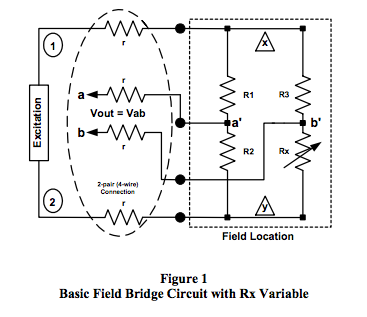
Analytical investigations throughout this document focus on the R-ohm type bridge, which means all bridge resistors are “R” ohms when not exposed to the field process variables. Figure 1 represents the R-ohm bridge type field sensor with all bridge resistors (R1, R2, R3, Rx) located at the point of field measurement; however, as resistor Rx is the bridge resistive sensor element, it varies with process parameters such as temperature, flow, pressure, level, humidity, strain, etc. In R-ohm bridge topologies, R1, R2, R3 are equal to R and Rx = (R+Δ R) where Δ R is a function of process variables.
Examples
Two categories of R-ohm bridge topologies will be examined. Category 1 bridges are defined as bridge topologies with all bridge resistors located in the field with one or more elements exposed to the process variable; Category 2 bridges are defined as having one or more bridge resistive sensor elements that are located in the field exposed to the process variables, with the remaining bridge resistors located at the point of electrical excitation. Bridges with one or two process variable elements are often referred to as quarter and half bridges, respectively.
Category 1 R-ohm Bridge with Voltage Excitation
This example is based on Figure 1 where the excitation source is voltage V12. The actual bridge excitation voltage, Vxy, is not constant because of voltage drops in the excitation line resistance. Bridge output voltage is Vout = (Va-Vb) = Vab. If Vab is always measured with a high impedance (typically > 1MΩ ) device, then sense line resistances can be neglected and Vab = Va’b’. As an example of the effects of sense line resistances, assume line resistance of 10Ω , voltmeter with 1MΩ input impedance, and a 120Ω bridge. The voltmeter loading on terminals a’-b’ is approximately 0.99988, whereas the loading on terminals a-b is approximately 0.99987 or a difference of -0.001%.
Equation 1 illustrates the output voltage, Vout = Vab, of Figure 1, neglecting all line resistances.
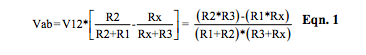
Equation 1 illustrates the classic bridge balance equation, which defines a set of resistor values that balances the bridge, resulting in zero bridge output voltage, Vab = 0. This condition occurs when R1*Rx = R2*R3. Note: The classic bridge balance condition is valid independent of line resistance and voltage excitation value. Clearly, this makes the bridge a useful circuit topology for balance measuring applications.
Christie’s 1833 paper showed that if Rx is an unknown and R2 = R1, then the bridge output will be zero (it was easy to measure zero in 1833) when R3 is adjusted to be equal to the unknown resistance, Rx. Many industrial transducers use bridge circuits with one or more bridge resistances that are functions of process variables such as temperature, flow, pressure, strain, humidity, etc. In these situations, bridge topology based transducers can not be conveniently (or economically) balanced at the field location; therefore, non-zero output bridge voltages are measured. Unlike balance measurements, bridge excitation and line resistances will contribute to measurement errors.
Industrial transducers with bridge circuit topologies have resistor sets that balance the bridge at a steady state value determined by a specific steady state field parametric input. As these steady state parameters change, the bridge becomes unbalanced and the output is non-zero. Measuring this unbalanced voltage with an appropriate scale factor applied is a direct indication of the change in field variable. The useful range of these voltages falls in the microvolt to millivolt category; consequently, low voltage measurement techniques must be utilized.
Equation 2 is the voltage output of R-ohm bridge circuit topologies shown in Figure 1, with voltage excitation including excitation line resistances.
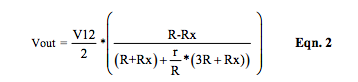
If excitation line resistances are negligible, this equation reduces to:
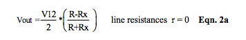
Figure 2 depicts the output response of the 120Ω bridge topology shown in Figure 1 to changes in Rx. In this simulation, the excitation is 5VDC, Rx ranges from 20Ω to 220Ω , and three different excitation line resistances – zero, 5Ω , and 20Ω – are used. Output line resistance is neglected, which is a valid technique, as previously shown.
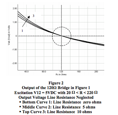
Figure 2 and Equation 2 reveal some important facts about Category 1 bridges.
Analytical investigations throughout this document focus on the R-ohm type bridge, which means all bridge resistors are “R” ohms when not exposed to the field process variables. Figure 1 represents the R-ohm bridge type field sensor with all bridge resistors (R1, R2, R3, Rx) located at the point of field measurement; however, as resistor Rx is the bridge resistive sensor element, it varies with process parameters such as temperature, flow, pressure, level, humidity, strain, etc. In R-ohm bridge topologies, R1, R2, R3 are equal to R and Rx = (R+Δ R) where Δ R is a function of process variables.
Examples
Two categories of R-ohm bridge topologies will be examined. Category 1 bridges are defined as bridge topologies with all bridge resistors located in the field with one or more elements exposed to the process variable; Category 2 bridges are defined as having one or more bridge resistive sensor elements that are located in the field exposed to the process variables, with the remaining bridge resistors located at the point of electrical excitation. Bridges with one or two process variable elements are often referred to as quarter and half bridges, respectively.
Category 1 R-ohm Bridge with Voltage Excitation
This example is based on Figure 1 where the excitation source is voltage V12. The actual bridge excitation voltage, Vxy, is not constant because of voltage drops in the excitation line resistance. Bridge output voltage is Vout = (Va-Vb) = Vab. If Vab is always measured with a high impedance (typically > 1MΩ ) device, then sense line resistances can be neglected and Vab = Va’b’. As an example of the effects of sense line resistances, assume line resistance of 10Ω , voltmeter with 1MΩ input impedance, and a 120Ω bridge. The voltmeter loading on terminals a’-b’ is approximately 0.99988, whereas the loading on terminals a-b is approximately 0.99987 or a difference of -0.001%.
Equation 1 illustrates the output voltage, Vout = Vab, of Figure 1, neglecting all line resistances.
Equation 1 illustrates the classic bridge balance equation, which defines a set of resistor values that balances the bridge, resulting in zero bridge output voltage, Vab = 0. This condition occurs when R1*Rx = R2*R3. Note: The classic bridge balance condition is valid independent of line resistance and voltage excitation value. Clearly, this makes the bridge a useful circuit topology for balance measuring applications.
Christie’s 1833 paper showed that if Rx is an unknown and R2 = R1, then the bridge output will be zero (it was easy to measure zero in 1833) when R3 is adjusted to be equal to the unknown resistance, Rx. Many industrial transducers use bridge circuits with one or more bridge resistances that are functions of process variables such as temperature, flow, pressure, strain, humidity, etc. In these situations, bridge topology based transducers can not be conveniently (or economically) balanced at the field location; therefore, non-zero output bridge voltages are measured. Unlike balance measurements, bridge excitation and line resistances will contribute to measurement errors.
Industrial transducers with bridge circuit topologies have resistor sets that balance the bridge at a steady state value determined by a specific steady state field parametric input. As these steady state parameters change, the bridge becomes unbalanced and the output is non-zero. Measuring this unbalanced voltage with an appropriate scale factor applied is a direct indication of the change in field variable. The useful range of these voltages falls in the microvolt to millivolt category; consequently, low voltage measurement techniques must be utilized.
Equation 2 is the voltage output of R-ohm bridge circuit topologies shown in Figure 1, with voltage excitation including excitation line resistances.
If excitation line resistances are negligible, this equation reduces to:
Figure 2 depicts the output response of the 120Ω bridge topology shown in Figure 1 to changes in Rx. In this simulation, the excitation is 5VDC, Rx ranges from 20Ω to 220Ω , and three different excitation line resistances – zero, 5Ω , and 20Ω – are used. Output line resistance is neglected, which is a valid technique, as previously shown.
Figure 2 and Equation 2 reveal some important facts about Category 1 bridges.
- Bridge output is sensitive to excitation line resistance and will always be sensitive to excitation voltage, V12.
- The bridge output voltage is nonlinear for nominal changes in Rx regardless of excitation line resistance and excitation voltage.
- As range of Rx decreases, the bridge output voltage begins to approach zero and appears to become more linear. See circle in Figure 2.
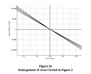
Figure 2a shows that the bridge output voltage still appears to be linear for very small variations of Rx and remains sensitive to excitation line resistance.
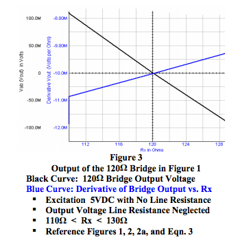
A question arises here. Is the voltage output of the bridge topology in Figure 1 ever linear? To answer this, Equation 3 is the partial derivative of the R-ohm bridge Vout in Equation 2a with respect to Rx (change in Vout for a change in Rx) with all other variables assumed constant and no excitation line resistance.
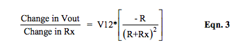
It is clear that Equation 3 is a nonlinear function and is not constant, which is the condition necessary for Vout to be a linear function of Rx. Thus, Figure 1 type bridge circuits cannot have outputs that are linear functions of Rx. See Figure 3.
For the range of Rx between 110 and 130 ohms, changes in Vout with changes in Rx (Equation 3 and Figure 3) range between -11.3 and -9.6mV per ohm with an average value of -10.5mV per ohm at balance.
Although these numbers are interesting, it is not practical to use partial derivatives in calculating bridge outputs. Common practice is to recognize that bridge circuits have nonlinear outputs, which are influenced by excitation line resistance, and to accept manufacturers’ specified transfer function data and installation instructions for their bridge sensors.
Category 1 R-ohm Bridge with Current Excitation
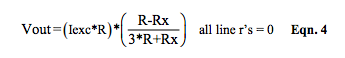
For well over a century, bridge topologies with voltage excitation have been used. Today, with modern semiconductor circuit technology, current source excitation is also an option. Equation 4 represents the output of a current, Iexc, excited R-ohm bridge (Figure 1) with output voltage line resistance neglected and no excitation line resistance.
Equation 4 becomes Equation 4a when the current excitation is adjusted to be Iexc = (V12 / R).
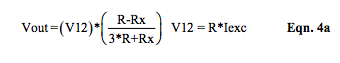
Note the similarity between Equations 2a and 4a.
Equation 5 is the partial derivative of the R-ohm bridge Vout in Equation 4a with respect to Rx (change in Vout for a change in Rx) with all other variables assumed constant.
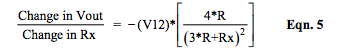
Where V12 = R*Iexc
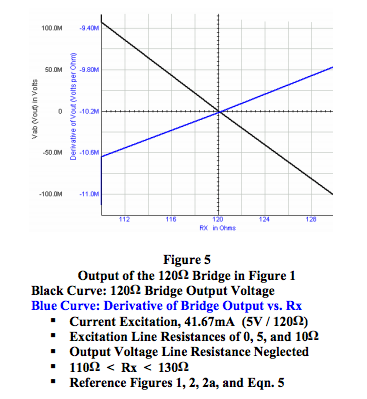
Figures 4 and 5 provide a visual comparison of the output voltages for the Category 1 R-ohm bridge with both voltage and current excitation.
Figure 4 illustrates the performance of a 120Ω bridge circuit as shown in Figure 1 with current source excitation at terminals 1 and 2 where line resistances are zero. The value of this current source was selected to be 41.667mA, which is 5VDC / 120Ω . This value of current provides 5VDC excitation at the bridge terminals when Rx is 120Ω , the condition of no field parametric inputs.
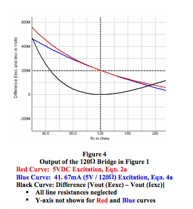
Figure 5 shows that the output behavior for the 120Ω bridge topology shown in Figure 1, with current excitation including different line resistances of zero, 5, and 10 ohms, is independent of excitation line resistances. In this case, the change in Vout for a change in Rx varies from -10 to -10.8mV per ohm with an average of -10.4mV per ohm, which is approximately the same as for voltage excitation but clearly still not constant.
Comparison of Category 1 R-ohm Bridge Excitations
The list of observations below are based on the 120Ω bridge topology of Figure 1 with either 5VDC voltage excitation or 41.67mA current excitation, with excitation line resistances of zero, 5, and 10 ohms included and output voltage line resistance neglected.
- Equations 4, 4a, and Figure 5 (Black Curve) show that for current excitation the output of the R-ohm bridge topology shown in Figure 1 is independent of excitation line resistance.
- Figure 4 shows that when line resistance is neglected the R-ohm 4-wire bridge output is more linear over a large range of Rx for current excitation (blue curve) than for voltage excitation (red curve).
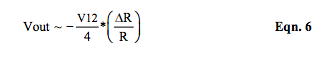
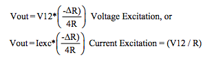
- Equation 6 and Figure 4 (black curve) show that the bridge outputs as illustrated by voltage excitation (Equation 2a) and current excitation (Equation 4a) are essentially identical near balance. Near balance, one can assume that R >> Δ R. Note that Rx = (R + Δ R) and Iexc is defined as V12 / R.
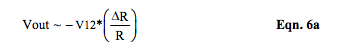
Interesting note: In Figure 1 type strain gage applications where changes in R1, Rx are positive equal and changes in R2, R3 are negative equal, Equation 6 becomes
Choosing Excitation
Excitation line resistances have different effects on bridge
output voltages depending upon which bridge category
(Category 1 or 2) and which excitation (current or
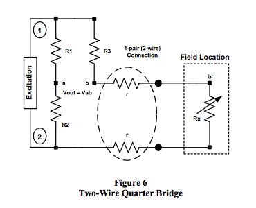
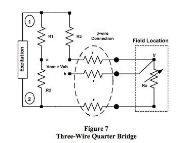
voltage) are used. Figures 6 and 7 illustrate the output
behavior of Category 2 R-ohm bridges with a single
bridge resistor located in the field connected to the
remainder of the bridge with two and three wires,
respectively.
Review
In the following Figure 1 bridge output voltage
expressions, R1 = R2 = R3 = R and Rx = (R+ΔR).
Voltage excitation is V12 and current excitation is Iexc
flowing into terminal 1. For convenience, behavioral
equations for the bridge shown in Figure 1 are revisited
here. Recall that voltage output line resistances are
neglected in Figure 1 and that Rx = (R + Δ R).
Figure 1 Equations (4-Wire Category 1)
Voltage excitation V12:
Current Excitation, with Iexc = V12 / R:
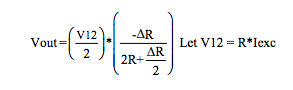
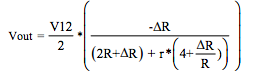
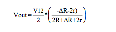
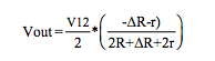
Figure 6 Equations (2-wire Category 2)
Voltage excitation V12:
Current Excitation, with Iexc = V12 / R:
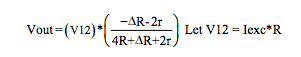
Figure 7 Equations (3-wire Category 2)
Voltage excitation V12:
Current Excitation, with Iexc = V12 / R:
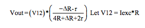
Figure 1 Equations (4-Wire Category 1)
Voltage excitation V12:
Current Excitation, with Iexc = V12 / R:
Figure 6 Equations (2-wire Category 2)
Voltage excitation V12:
Current Excitation, with Iexc = V12 / R:
Figure 7 Equations (3-wire Category 2)
Voltage excitation V12:
Current Excitation, with Iexc = V12 / R:
Conclusions
The following observations are made based on Figure 6
and Figure 7 topologies:
- Bridge voltage outputs are nonlinear regardless of whether current or voltage excitation is used.
- Category 1 bridge topologies have output voltages that are independent of line resistances when current excitation is used.
- Category 2 bridge topologies have output voltages that are always dependent on line resistances regardless of whether current or voltage excitation is used.
- If
 i.e., if line resistances can always
be neglected and if changes in the sense resistor Rx are
very small compared to R, then bridge output is the
same for voltage or current excitation.
i.e., if line resistances can always
be neglected and if changes in the sense resistor Rx are
very small compared to R, then bridge output is the
same for voltage or current excitation.
Output responses for R-bridge circuits containing more
than one variable resistive element, with equal but
opposite changes to process variables, are common in
strain gage bridge circuits. These circuits are discussed in
Dataforth’s application note on strain gages.
Figure 8 is a block diagram of Dataforth’s Bridge Signal Conditioning Module Series SCM5B38. These modules are designed to interface with Category 1 full bridge circuits with options for Category 2 half and quarter bridge topologies. This module’s predominant application is in industrial strain gage instrumentation applications; however, it is well-suited for any bridge type instrumentation application.
Dataforth’s bridge SCMs SCM5B38 (Narrow BW), SCM5B38 (Wide BW), and DSCA38 have multiple (typically 5-7) pole filters with anti-alias filtering on the field side. Moreover, these modules have 4-way isolation, which includes precision isolated voltage for field excitation, isolated field-side power, isolated computer-side power, and signal isolation. Dataforth’s DIN rail DSCA38 series of modules has both narrow and wideband filter options to accommodate a wide range of applications. In addition, the DSCA38 series has +/-5% front-panel adjustments for zero and span. Zero adjustments are particularly useful for balancing bridge circuits. The reader is encouraged to visit Dataforth’s website, Reference 1, and examine all the options for the SCM5B38 and DSCA38 bridge modules, as well as Dataforth’s complete line of SCMs.
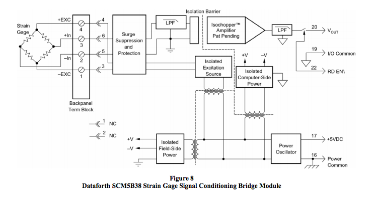
Dataforth References
1. Dataforth Corp., http://www.dataforth.com
Was this content helpful?
Thank you for your feedback!