

AN115: Sampling Law
Application Note
Preamble
Information that varies continuously as a function of time is analog information. Computers are digital devices and, therefore, must convert analog information to a digital format in order to work with the information. The analogto- digital conversion concept is fundamentally straightforward: Analog-to-digital circuitry interrogates (samples) analog signals at some periodic rate, converts each sample to a digital number, and then presents the individual samples to the computer as a representation of the time varying analog signal.A similar process is utilized in hardwire data acquisition and control systems, where it is necessary to physically isolate analog signals. Signal isolation is often required to eliminate troublesome grounding and noise problems; in such situations, “sampling concepts” are used to “transmit” the analog signal across a physical barrier.
Regardless of where sampling is used, one must consider the sampling rate. Reconstructed signals from these samples must adequately represent the original analog signal. Obviously, sampling too slowly (10Hz signal sampled every 30 minutes, for example) could lose valuable information, while sampling too fast (10Hz signal sampled at 300MHz) creates serious circuit problems. Fortunately, there is an answer to the sampling rate question. Figure 1 illustrates a typical sampling process.
The Law
Regardless of its original characteristics, data is stored by modern acquisition systems in digital form. Therefore, analog information must first be transformed to its digital equivalent using an analog-to-digital converter (ADC). In this type of system, the sample rate MUST exceed the highest frequency contained in the “detectable” input signal. This is not an option; it’s the law! In fact, the Nyquist criterion (part of the law) demands that we sample at greater than twice the highest frequency applied to the ADC. This is required to avoid aliasing, which may result in severe errors.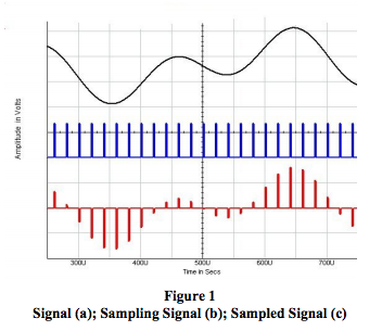
Nyquist defines the minimum sample rate required to yield meaningful information about a signal’s frequency content. Fourier analysis gives us the necessary tools to relate the amplitude of each frequency component to a given waveform. Given this information and proper signal processing, the original amplitude versus time (timedomain) waveform can be reconstructed.
Normally, software products are designed to display timedomain data in its original, unprocessed form. The result is that sine-like waveforms can be misrepresented by triangular-looking shapes. This is a presentation problem. The underlying data is not at fault. In these cases, presentation fidelity can be improved by sampling beyond the Nyquist requirement.
Sometimes, the underlying physical properties of the input transducer will define a maximum frequency response. In other applications, the Nyquist rule is enforced by inserting a low-pass filter to block undesired high frequencies. In either case, all frequencies that exceed half of the sample rate must be attenuated below the level that is detectable by the ADC.
Ideally, a device used to limit bandwidth would make a perfect distinction between wanted and unwanted frequencies. In the real world, however, filter components make a relatively gradual transition from the pass-band to the stop-band. The dividing line or transition point is often referred to as the corner frequency or f1 .
Figure 2 shows the response curves for a few practical filters. Note that while the rate of attenuation (slope of the curve beyond the corner frequency) can be quite steep, a portion of the unwanted frequencies still “leaks” past the filter. Assume for a moment that the input signal consists of all frequencies from DC to infinity and that the amplitude of each frequency is equal to the full-scale range of the ADC. Consider that an 8-pole Bessel filter is being used with a 12-bit ADC, and that f1 is set at 1kHz. Nyquist says that we can sample at 2kHz, right? WRONG! The sensitivity of a 12-bit converter is approximately -72dB. Therefore, frequencies beyond 6kHz can still be detected. As a result, the required minimum sample rate is 2 * 6 kHz = 12 kHz. Please remember – Nyquist does not care about the corner frequency of the filter or our highest frequency of interest. Only the highest detectable frequency counts.
Anti-aliasing filters can be classified in several ways. Most important are gain error in the pass-band, minimum attenuation beyond a given frequency in the stop-band (related to the resolution of the companion ADC), and time delay (phase shift versus frequency). For a given type, the number of poles determines the rate of attenuation in the stop-band. Table 1 suggests the minimum sampling frequency for several filter configurations. The numbers shown are to be multiplied by the filter’s f1 and then by 2 (for Nyquist). Note the significance of different ADC resolutions. What kind of filter (Bessel, Elliptic, etc.) should be used? Both Table 2 and Figure 2 offer some guidelines.
What about digital filters? Digital filters perform their function by mathematical manipulation of the acquired data. This simulates a physical filter. They are very useful in many types of noise reduction and spectrum modification applications. However, they can never be used for anti-aliasing purposes. Aliasing occurs in the analog-to-digital converter. As a general rule, no amount of digital processing can correct the damage done.
SUMMARY
- Steps must be taken to ensure that the sample frequency exceeds 2 times the highest detectable input frequency.
- A low-pass (anti-alias) filter is often used to limit the input spectrum.
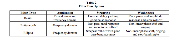
- The Bessel filter has linear phase shift as a function of frequency. This provides accurate response in both the time and frequency domains and can be used with pulse inputs. However, pass-band gain error can be significant near f1.
- The Elliptic filter is most efficient for fast, stop-band frequency rejection. However, the non-linear phase shift results in time-domain waveform distortion. This limits its use to the frequency domain.
- As a general rule, “better” filters have more poles. More poles cost more money.
- Adhering to the Nyquist rule ensures that aliasing will not occur and that accurate frequency-domain information will be preserved. However, even higher sample rates are required to record meaningful timedomain information.
- Unless the physical characteristics of the system (transducer and signal conditioner) inherently limit the signal bandwidth to under half of the sampling frequency, you need an anti-aliasing filter. If you think otherwise, you are probably wrong.
For a more in-depth review on anti-aliasing filter theory, see Microchip’s Application Note AN699, Reference 2.
Remember, don’t alias! It’s the law!
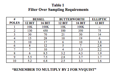
Figure 2 illustrates the response versus frequency attributes of three common filters.
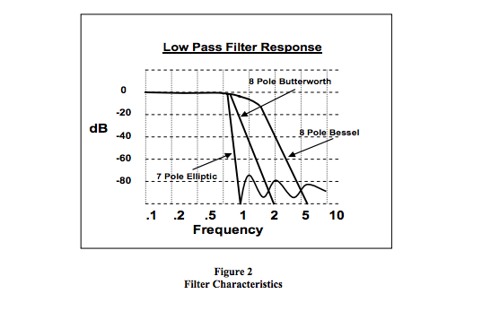
Table 2 illustrates the application, strengths, and weaknesses of the filters shown in Figure 2.
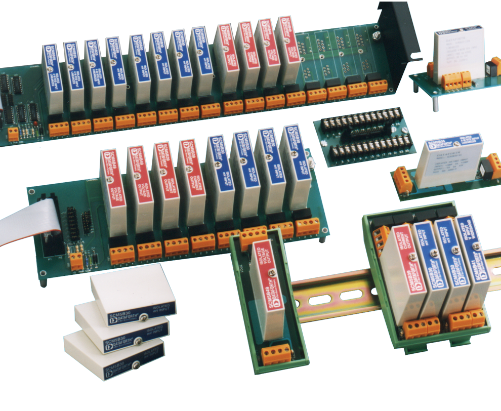
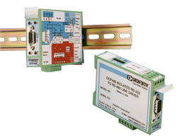
Dataforth’s design engineers include anti-aliasing filtering on the field side of their isolated SCMs, many of which have up to seven poles of filtering. As an example, the DSCA38 DIN isolated analog signal conditioning module for strain gages has 4- way isolation, which includes signal isolation with isolated power for the field side, system side, and sensor excitation. A 5- pole filter with an anti-aliasing section on the field side is included. Readers are encouraged to visit Dataforth’s website (Reference 1) and examine the complete line of SCMs.
Dataforth References
- Dataforth Corp.
https://www.dataforth.com - Microchip Technology, Chandler, AZ Anti-Aliasing, Analog Filters for Data Acquisition Systems (http://ww1.microchip.com/downloads/en/AppNotes/00699b.pdf)
Was this content helpful?
Thank you for your feedback!