


Measuring RMS Values of Voltage and Current (AN101)
Application Note
VOLTAGE (CURRENT) MEASUREMENTS
Standard classic measurements of voltage (current) values are based on two fundamental techniques either "average" or "effective".The "average" value of a function of time is the net area of the function calculated over a specific interval of time divided by that time interval.
Specifically,
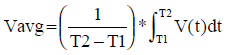 (Equation 1)
If a voltage (current) is either constant or periodic, then measuring its average is independent of the interval over which a measurement is made. If, on the other hand, the voltage (current) function grows without bound over time, the average value is dependent on the measurement interval and will not necessarily be constant, i.e. no average value exists. Fortunately in the practical electrical world values of voltage (current) do not grow in a boundless manner and, therefore, have well behaved averages. This is a result of the fact that real voltage (current) sources are generally either; (1) batteries with constant or slowly (exponentially) decaying values, (2) bounded sinusoidal functions of time, or (3) combinations of the above. Constant amplitude sinusoidal functions have a net zero average over time intervals, which are equal to integer multiples of the sinusoidal period. Moreover, averages can be calculated over an infinite number of intervals, which are not equal to the sinusoidal period. These averages are also zero. Although the average of a bounded sinusoidal function is zero, the "effective" value is not zero. For example, electric hot water heaters work very well on sinusoidal voltages, with zero average values.
EFFECTIVE VALUE
The "effective" value of symmetrical periodic voltage (current) functions of time is based on the concept of "heating capability". Consider the test fixture shown in Figure 1.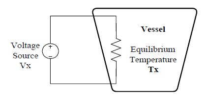
Figure 1: Test Fixture
This vessel is insulated and filled with some stable liquid (transformer oil for example) capable of reaching thermodynamic equilibrium. If a DC voltage Vx is applied to the vessel’s internal heater, the liquid temperature will rise. Eventually, the electrical energy applied to this vessel will establish an equilibrium condition where energy input equals energy (heat) lost and the vessel liquid will arrive at an equilibrium temperature, Tx degrees.
Next in this experimental scenario, replace the DC voltage source Vx with a time varying voltage which does not increase without bound. Eventually, in some time Tfinal , thermal equilibrium will again be established. If this equilibrium condition establishes the same temperature Tx as reached before with the applied DC voltage Vx, then one can say that the "effective" value of this time varying function is Vx.
Hence the definition of "effective value". Equation 2 illustrates this thermal equilibrium.
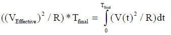 (Equation 2)
If V(t) is a periodic function of time with a cycle period of Tp, and Tfinal is an integer "n" times the period (n*Tp) then the integral over Tfinal is simply n times the integral over Tp. The results of these substitutions are shown in Equation 3.
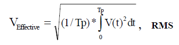 (Equation 3)
Equation 3 illustrates that the effective equivalent heating capacity of a bounded periodic voltage (current) function can be determined over just one cycle. This equation is recognized as the old familiar form of "square Root of the Mean (average) Squared"; hence, the name, "RMS".
EXAMPLES OF USING THE "RMS" EQUATION
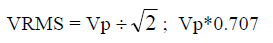
The following results can be shown by direct application of Eqn 3.- Sinusoidal function, peak of Vp
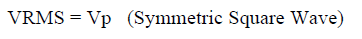
- Symmetrical Periodic Pulse Wave, peak of Vp
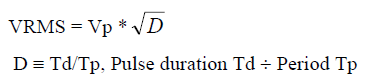
- Non-symmetrical Periodic Pulse Wave, all positive peaks of Vp, with duty cycle D
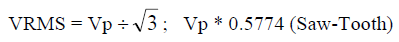
- Symmetrical Periodic Triangle Wave, peak Vp
- Full wave Rectified Sinusoid, peak Vp
- Half Wave Rectified Sinusoid, peak Vp
EFFECTIVE (RMS) VALUES OF COMPLEX FUNCTIONS
An extremely useful fact in determining RMS values is that any well behaved bounded periodic function of time can be expressed as an average value plus a sum of sinusoids (Fourier’s Theorem), for example;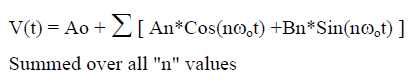 (Equation 4)
Where ωo is the radian frequency of V(t) and An, Bn, Ao are Fourier Amplitude Coefficients.
When this series is substituted in the integral expression Equation 2 for RMS, one obtains the following;
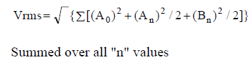 (Equation 5)
Note: (An)2 and (Bn)2/2 are the squares of RMS values for each nth Sin and Cosine component.
The important conclusion is;
A bounded periodic function of time has a RMS value equal to the square root of the sum of the square of each individual component's RMS value.
PRACTICAL CONSIDERATIONS
Figure 2 illustrates composite curves formed by adding two sinusoids, one at 60 Hz and one at 180Hz. Curve 1 is for zero phase difference and Curve 2 is for a 90-degree phase difference.Specifically;
Curve 1 V(t) = 170*Sin(377*t) +50*Sin(1131*t)
Curve 2 V(t) = 170*Sin(377*t) +50*Cos(1131*t)
Note: Composite curve shape is determined by phase and frequency harmonics.
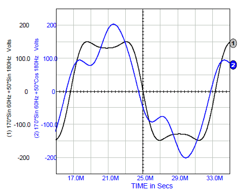
Figure 2: Fundamental with Third Harmonic Added
Curve 2 170*Sin(377*t) +50*Cos(1131*t)
Curve 1 170*Sin(377*t) +50*Sin(1131*t)
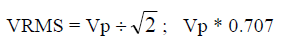
Industrial sinusoidal functions of voltage (current) often contain harmonics that impact wave shape and peak (crest) values. For example, Curve 2 is typical of the magnetizing currents in 60 Hz transformers and motors. Inexpensive RMS reading devices often use a rectifier circuits that capture the peak value, which is then scaled by 0.707 and displayed as RMS. Clearly this technique can give incorrect RMS readings. In this example, using Vpeak ÷√2 clearly gives incorrect values.
Curve 1: 203*0.707 = 144 volts, not true RMS
Curve 2: 155*0.707 = 110 volts, not true RMS
The correct RMS value for both of these composite sinusoidal functions is;
[ (170)2/2 + (50)2/2 ]1/2 = 125.3 volts RMS
Table 1 illustrates two examples of RMS calculations by using individual Fourier coefficients and Eqn 5. Example one is a full wave rectified 1-volt peak sinusoid. Note that for a full wave rectified function the measurement device needed to achieve a RMS reading within 0.01% error requires a bandwidth, which includes the fifth (5) harmonic and the resolution to read 10 mV levels. The other example illustrated in Table 1 is a saw-tooth 1-volt peak function. For this example, the measurement device for a saw-tooth function needed to achieve an RMS reading within 0.3% error requires a bandwidth, which includes the twenty-fifth (25) harmonic and the resolution to read 10 mV levels.
Assume, for illustration purposes, that an AC ripple on the DC output of a rectifier can be approximated by a saw-tooth function. Table 1 illustrates that to measure within a 0.3% error the AC RMS ripple on the DC output of a 20 kHz rectifier the measurement device must have a bandwidth in excess of 500 kHz and a resolution to read voltage levels down by 40 dB (100 microvolts for a peak 10 mV ripple). This example clearly illustrates that signal shape, together with the measurement bandwidth and resolution are extremely important in determining the accuracy of measuring true RMS.
Any "true RMS" measurement device must be capable of accurately implement Eqn 3. The subtlety in this statement is that electronically implementing Eqn 3, requires a device to have a very large bandwidth and be able to resolve small magnitudes.
CREST FACTOR
Another figure of merit often used to characterize a periodic time function of voltage (current) is the Crest Factor (CF). The Crest Factor for a specific waveform is defined as the peak value divided by the RMS value. Specifically,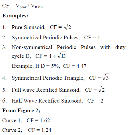
DATAFORTH RMS MEASUREMENT DEVICES
True RMS measurements require instrumentation devices that accurately implement Eqn 3, "the" RMS equation. These devices must have both wide bandwidths and good low level resolution to support high Crest Factors. Dataforth has developed three products that satisfy these requirements; the SCM5B33, DSCA33, and 8B33 True RMS Input modules. These products provide a 1500Vrms isolation barrier between input and output.


Was this content helpful?
Thank you for your feedback!