an114: Accuracy versus Resolution

Preamble

System error budgets should be developed and analyzed as an integral part of system designs. System engineers must determine the necessary levels of accuracy for system elements such as field sensors, actuators, signal conditioning modules (SCMs), and controlling units (PCs and PLCs). In addition, software algorithm integrity and operating system compatibility, or the degree of software “openness,” must be included in error budget considerations. For example, the accuracy and resolution of software algorithm calculations must be compatible with measurement accuracy.

In the process of analyzing system accuracy needs, the topic of resolution requires attention as it relates to overall accuracy. Oftentimes distinguishing between accuracy and resolution is misinterpreted in determining system needs. Some examples and illustrations are presented in this Application Note in an attempt to show readers that there is a significant difference between accuracy and resolution, even though they are related.

Examples

Before launching into some examples, recall how accuracy is denoted. A reading device that has a specified accuracy of ±0.015% will actually give a reading that is between 0.99985 and 1.00015 times the actual value. Interesting how our standards have defined “accuracy.” Note here that the ±0.015% number is in reality the “error.”

Accuracy is the measurement device’s degree of absolute correctness, whereas resolution is the smallest number that can be displayed or recorded by the measurement device. For example, measuring 1 volt within ±0.015% accuracy requires a 6-digit instrument capable of displaying five decimal places. The fifth decimal place represents 10 microvolts, giving this instrument a resolution of 10 microvolts.

For the following examples, the digital display quantizing error (±1 bit minimum) in the least significant digit is assumed to be zero.

Example 1
Suppose one has a voltage source that is known to be exactly 5.643 volts. Now imagine, if you will, that one uses a digital voltmeter that is (somehow) 100% accurate, but has only 3 display digits and is defined as “3-digit resolution.” The reading would be 5.64 volts. Is the reading accurate? There was an accurate source and an accurate voltmeter, yet the reading does not represent the actual voltage value. Some may say that our 100% accurate voltmeter gave us a reading error of 3 millivolt or 0.0532%.

In this hypothetical example, the reading could be considered in error unless one only wants a 3-digit reading. In cases where source and instrument accuracy are 100%, the resolution of the reading instrument and the acceptance of the observer determine what constitutes “accuracy.”

Example 2
Again assume a 100% accurate source of 5.643 volts; however, in this case our 3-digit display digital voltmeter has a ±0.015% accuracy specification (recall this means that the displayed value is actually between 0.99985 and 1.00015 times the source value).

In this case, the digital voltmeter still reads 5.64 volts. One can say that this 0.015% accurate instrument gives a 0.0532% error, as in Example 1. Once again, the resolution and the observer determine what constitutes “accuracy.”

Example 3
In this example, consider measuring the precise 5.643- volt source using a 5-digit display digital voltmeter with a specified accuracy of ±0.015%. This instrument displays a reading of between 5.6421 (for 5.64215) and 5.6438 (for 5.64385).

Example 4
Repeat Example 3 using a 6-digit display digital voltmeter, again with a specified accuracy of ±0.015%. The display will be between 5.64215 and 5.64385.

Clearly, these examples illustrate that accuracy and resolution are indeed related, and each situation has to be evaluated based on the system requirements and the observer’s acceptance of “error.”

Reality

A typical situation is illustrated in Figure 1. As shown, sensor signals are conditioned with signal conditioning modules, selected, and then converted into a usable number either for analytical process control or observation.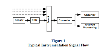



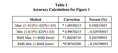
In Figure 1, assume sensors have ±0.25% (E1) accuracy specifications, SCMs have ±0.03% (E2) accuracy specifications, and the select-converter function has ±0.05% (E3) net accuracy. Table 1 displays some different system “accuracy” correction calculations. Since errors are random and have ± values, RMS calculations are often used as opposed to the worst case maximum and minimum. RMS error is defined as the square root of the sum of each error squared, √ {(E1)2 + (E2)2 + (E3)2 }.



Number values from the converter function in Figure 1 are presented to the observer with a display unit that has its own error and resolution specifications. In addition, the analytical processing function imports this numerical value to use in a complex mathematical operation, which may be based on an empirical model that achieves results using computation shortcuts, which in turn have additional accuracy and resolution specifications.

As is evident, a detail error budget must contain numerous factors in order to correctly determine “system accuracy.”

Reality Check
Have you ever experienced this scenario or one similar?

Analog-to-digital converters (ADC) are advertised as having “n” bit resolution, which often is misunderstood to mean accuracy. Specifications need to be closely examined, however, to determine the unit’s true accuracy.

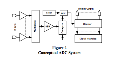
Figure 2 depicts one typical scheme used to convert an analog signal to a digital representation for computer manipulations or display. In this typical representation, semiconductor switches select analog input signals, which are captured (sampled for a small slice of time) and held in a sample and hold amplifier function block (SHA). This SHA function may also contain a programmable gain function to selectively scale each analog input. Once a signal slice is captured, an n-bit counter begins to count. The counter contents are converted to an analog voltage using switched resistors or current sources. When this analog signal equals the input SHA signal, counting halts and the counter contents are made available as a digital representation of the sampled analog input value. This process can sample analog inputs at blinding speeds in the 10MHz range to provide digital representations of time varying analog inputs; it also has numerous sources of error that collectively degrade true accuracy, which is not necessarily determined solely by the n-bit resolution specification.



ADC Error Budget
The following list identifies errors associated with using a typical ADC scheme such as illustrated in Figure 2.

1. Sampling Speed
   From Nyquist Sampling Theory, if the analog signal changes rapidly, then the ADC must sample at least twice as fast as the changing input. Many applications use a sampling rate at least 10 times the highest frequency present in the input signal. Sampling slower than one-half the signal frequency will result in inaccurate readings. Most ADC’s sampling speeds are adequate for slow varying process control signals. See Reference 2 for more details on this topic.


2. Input Multiplexed Errors
   The input multiplexer circuit may have OpAmp buffers on each input line that could introduce errors such as in voltage offset, current bias, and linearity. In addition (and more common) are the two major multiplexer errors: (a) cross talk between channels, i.e., the signal from an “on” channel leaks current into the “off” channels, and (b) signal reduction through voltage division caused by the finite non-zero resistance of the semiconductor switches and the finite input impedance of the circuitry that follows.


3. Sample and Hold Amplifier (SHA)
   This function is an OpAmp based circuit with capacitive components all designed to switch, buffer, and hold the sampled analog voltage value. Consequently, there will be linearity, gain, powersupply rejection ratio (PSRR), voltage offset, charge injection, and input bias current errors. For a detail analysis of typical OpAmp errors, see Dataforth’s Application Note AN102, Reference 3.


4. Converter
   In the counter, comparator, and ADC circuit there are such errors as overall linearity, quantizing error (defined as uncertainty in the least significant bit [LSB], typically ±1/2 LSB), and PSRR.


5. Temperature
   All analog circuit functions within the ADC unit are subject to temperature errors and hence an overall temperature error specification is assigned to an ADC.

Table 2 identifies some of the internal errors associated with a typical ADC. Data was taken from various analogto-digital converter manufacturers. This table is by no means a complete ADC error analysis; the values shown illustrate that there are internal errors that collectively contribute to the definition of an ADC’s overall accuracy.



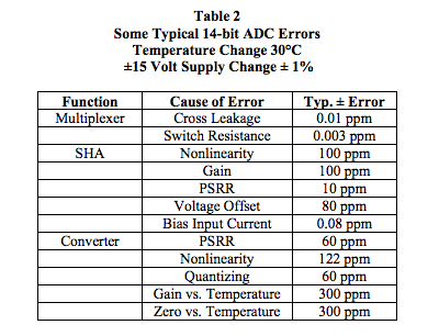
An algebraic sum model on these errors suggests a ±0.1% error for this 14-bit ADC, whereas the RMS sum model suggests a ±0.05 % error. Resolution alone erroneously implies ±0.006%. These internal ADC error numbers used in either an algebraic or RMS summing model clearly illustrate that the net effective accuracy of an n-bit ADC is not equal to the ADC resolution, defined as approximately 1/(2n -1). To determine actual ADC accuracy, the manufacturer’s ADC specifications should always be carefully examined.

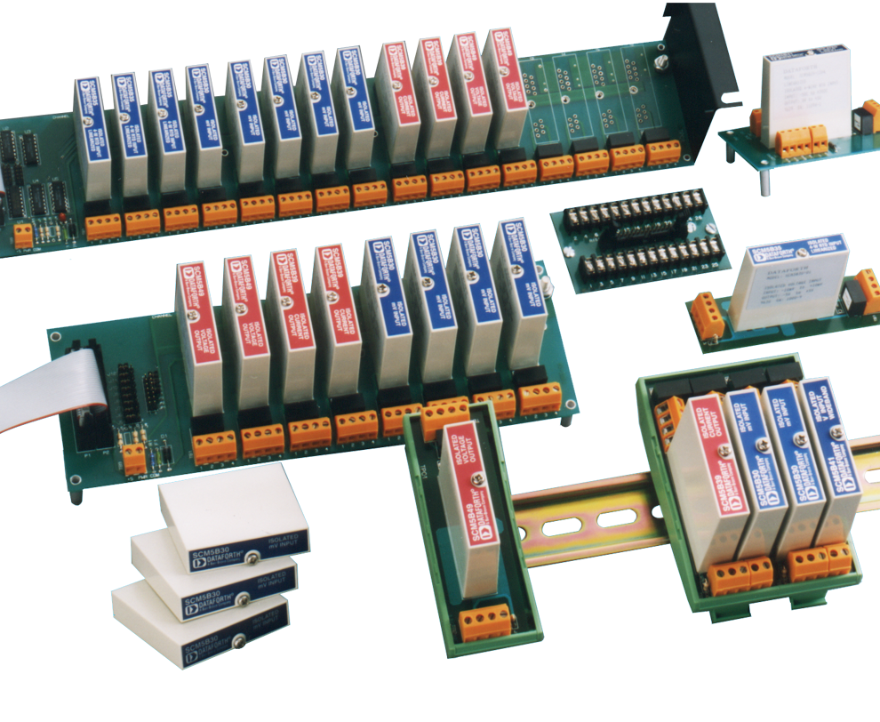
Note: Industrial sensors used in process control and data acquisition systems can have accuracies that are much less than SCMs or ADC units and often dominate errors in a total system error budget. Dataforth SCMs have accuracies that typically exceed both those of industrial sensors and ADC modules. Readers are encouraged to examine Dataforth’s complete line of SCM products. See Reference 1.

Dataforth References

1. Dataforth Corp. Website
   http://www.dataforth.com
2. Dataforth Corp., Application Note AN112
   http://liwww.dataforth.com/technical_lit.html
3. Dataforth Corp. Excel Interactive Workbook for 2-Pole LP Active Filter
   http://liwww.dataforth.com/catalog/pdf/an113.xls