an112: Filtering in Signal Conditioning Modules, SCMs

Preamble

Signal conditioning modules, SCMs, used for measuring process control variables such as temperature, pressure, strain, position, speed, level, etc. are always subject to externally induced noise signals. Electrically and magnetically induced noise voltages/currents are inevitable. Field sensors with output voltages in the millivolt range are certainly degraded by induced noise levels on the order of volts. Consequently, signal conditioning modules must provide filtering to eliminate induced noise components.

Hundreds of articles and text books have been written on filters that provide a multitude of frequency characteristics such as the Bessel, Butterworth, Chebyshev, Cauer, etc. In-depth reviews of this information are beyond the scope and intent of this document. The objective of this application note is a brief review of filter fundamentals primarily focused on the amplitude response of low-pass (LP) filters needed in industrial signal conditioning modules.

Brief Review of Some Fundamentals

Filter topologies are characterized by their transfer functions, which are frequency dependent ratios of output voltage (Vout) to input voltage (Vin) expressed as ratios of polynomials as shown. For example,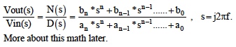



Filter transfer function behavior is generally characterized by “Bode” plots, which are semilog plots of phasor amplitudes in decibels {20*log (Vout/Vin)} versus frequency and semilog plots of phasor phases in degrees versus frequency.

Figure 1 illustrates Bode magnitude plots of three fundamental RC filter types; curve #1 single section RC low-pass (LP) filter, curve #2 single section high pass (HP) filter, and curve #3 two section bandpass filter.



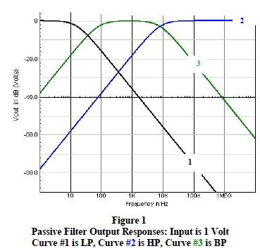
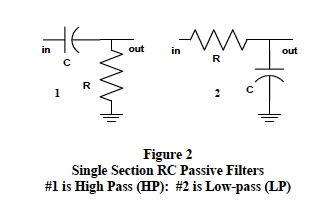
Low-Pass (LP) filters allow transmission of only a range of low frequencies from DC to a higher cutoff frequency. See Figure 2, circuit #2 and Figure 1, curve #1. This type of filter is ideal for eliminating high frequency induced noise on low frequency signal data. Low-Pass filtering is required in most industrial SCMs to eliminate induced 60 cycle harmonics and randomly induced high frequency transient noise.

High-Pass (HP) filters allow transmission of a range of high frequencies from a lower cutoff frequency to an upper limit of circuit component performance. See Figure 2, circuit #1 and Figure 1, curve #2 . These type filters are ideal for eliminating induced low frequency noise on high frequency signal data.

Bandpass (BP) filters allow transmission of a range of frequencies between a lower and upper cutoff limit. The characteristics of a simple BP filter are shown in Figure 1, curve #3 and can be simulated by cascading the HP and LP circuits in Figure 2. These type filters are ideal for signal selection within a given frequency range. Conversely, bandpass filter transfer functions can be rearranged to function as “notch” filters, which eliminate frequencies between a lower and upper cutoff limit.

Basic Filter Characteristics

Traditional filter transfer functions are implemented with either passive or active circuit topology. Passive filter circuit topology is configured with individual resistors, capacitors, and inductors; whereas, the typical active filter circuit uses operational amplifiers with resistors and capacitors in various feedback arrangements. Unique filter transfer function characteristics are implemented with active filters by selecting resistor and capacitor values in the feedback topology and by adjusting the filter’s amplifier gain. Some basic SCM filtering characteristics are illustrated in the following list.

Bandpass: This filter transfer function applies equally to all frequencies within the range (band) of desired filtering with no amplitude variations within in the filter’s desired bandpass (i.e. a flat response with no ripples). Frequency components outside the bandpass are sharply attenuated. See Figure 1, Curve #3.

Sharp Response at Cutoff Frequencies: Frequencies where the filter’s power response has dropped 50% or 1/√ 2 (0.707) of the desired output voltage are defined as “cutoff” frequencies. Bode plots locate these cutoff frequencies 3 decibels below the flat mid range; hence, the term “3-dB points”. Ideal filters have no response below their lower 3-db cutoff, no response above their upper 3-dB cutoff, and very steep response slopes approaching these 3-dB points. The term “bandwidth” defines the frequency range between 3-dB “cutoff” frequencies. For low-pass filters, the bandwidth is from DC to the 3-db frequency. See Figure 1, Curve #1.

Note 1: Analysis on LP filters shows that cutoff behavior near 3-dB frequencies is determined by a mathematical combination of the individual roots (called “poles”) of the filter transfer function denominator polynomial, D(s). These roots are functions of the time constants within a filter circuit and have the units of Hz or radians/sec. The number of roots (order of denominator polynomial) is equal to the number of circuit time constants. For example, a RC low-pass filter containing four capacitors has four RC time constants and a fourth order denominator polynomial with four roots (poles).

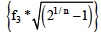
The mathematical combinations of denominator roots and the frequency spread between them determine the actual 3-dB frequency. For instance, if all the individual roots differ by a factor of 10 then the lowest root (largest time constant) essentially is the 3-dB point. On the other hand if a filter has “n” equal roots, then the 3-dB point is



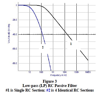
For situations between these two simple extremes, the math becomes complicated and computer simulations with bench testing are more effective ways to determine 3-dB points. Figures 3 and 6 illustrate the effects multiple poles have on “the” 3-dB frequency.

Note 2: Continued analysis of LP filter transfer functions reveals that the number of roots (or number of filter time constants) controls the slope of a filter’s response as it approaches the 3-dB point. Beyond the cutoff frequency, each pole contributes an amplitude decrease of 20 dB per frequency decade to the filter response. For example, a 4- pole filter response beyond the 3-dB point has a limiting slope of -80 dB per decade.

Figure 3 and Figure 6 illustrate the effect of multiple poles (RC sections) for a low-pass filter.


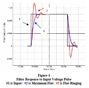
Over shoot: Sensors often output step functions or near instantaneous transitions between signal levels. SCM filters should not allow excessive overshoot or ringing in responses to these step functions. RC time constants and filter gain determine active filter overshoot. Figure 4 shows the effects of modifying active filter time constants and gain.

Filter Response Calculations

Manual analysis of filter transfer functions is laborious and best implemented with special computer application programs; nonetheless, many salient filter characteristics are illuminated by manual analysis of simple filter topologies using Steinmetz’s phasor concepts and Laplace transformations.

As an example consider the simple 2 RC section passive LP filter topology shown in Figure 5. The fundamental time dependent behavioral loop equations for this circuit are;



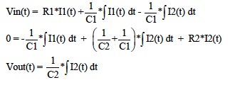
Transfer function (Vout/Vin) derivations from these equations require considerable effort. Using phasor definitions, Laplace transformations, and steady-state frequency dependent sinusoidal voltages, reduce this effort to simple algebraic equations where Laplace transformation allows “s” to represents the complex frequency term “jω ”. The LP filter transfer function time dependent equations for Figure 5 now become;



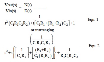
Note: D(s) in both these equations is a quadric denominator of the form ( a*s2 + b*s + c ) with two roots.



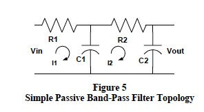
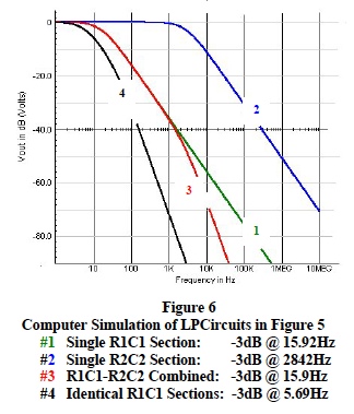
As an example, choose Figure 5 component values to be; R1=20kΩ , C1=0.5μF, R2=56kΩ , and C2= 0.001μF. A computer simulation program that sweeps the input sinusoidal voltage from one hertz to ten megahertz generates the results shown below in Figure 6.



Further examination of this example, illuminates some important fundamental low-pass filter characteristics.

• Each separate low-pass RC section has a cutoff frequency (response down by 3-dB) related to their individual RC time constant. Recall that for a single RC LP section the cutoff frequency f3 is 1/ (2π RC) Hz. See Figure 6, curve #1 and curve #2 Low-pass filters with identical RC sections have a much lower cut off frequency than the individual RC section. See curve #4 in Figure 6.
• Each single low-pass RC section contributes a 20 dB change in voltage response for each factor of 10 change in frequency (20dB per decade). Recall that a 20 dB change represents a factor of 10 change in voltage ( i.e. a voltage change from 1 to 0.1 is a – 20 dB change). As RC sections with near equal time constants are added, the cutoff frequency decreases and, most importantly, the response slope increases. For example, one RC section gives 20 dB / decade whereas five RC sections give 100dB/ decade slope. SCM filters need low cutoff frequencies with steep rates of response to ensure effective rejection of noise beyond the LP cutoff.
• The quadric denominators “D(s)” in Eqn.1 and Eqn. 2 have identical roots; 15.71 Hz and 2.8794 kHz. The denominator “roots” of these RC filter transfer functions are determined by circuit RC time constants and are defined as “poles”, which control the filter’s cutoff frequency. The above example illustrates a fundamental filter characteristic; namely, low-pass RC filter cutoff frequencies are dominated by the smallest pole. See curve #3 in Figure 6
• Low-pass RC filter transfer functions, which are arranged as shown in Eqn 1, always have denominators with “b”, the coefficient of the first power of “s” equal to the sum of the filters “open circuit” time constants and the filter cutoff frequency can be estimated by 1/(2πb). In Figure 5, the sum of open circuit time constants is [R1C1 + C2*(R1+R2)] = 10.076mS and frequency associated with this time constant is 15.8 Hz. Recall that; frequency is related to a time constant “T” by the expression [f=1/(2*π *T)] and that an open circuit time constant is the product of each capacitor and the effective resistor this capacitor “sees” with all other capacitors open. Open circuit time constants are referred to by the mnemonic “OCTs.”
• The numerators “N(s)” of valid filter transfer functions, N(s)/D(s), force the filter response to zero and are defined as filter “zeros”. Low-pass SCM filters have no “zeros”
• Filter transfer functions have frequency dependent phase shifts and time delays, both of which are extremely crucial in high frequency communication applications. Substituting s = j2π f in Eqn 1 and 2 illustrates frequency dependent phase angles. Phase characteristics of SCMs in industrial data acquisition systems are not generally an issue but may be crucial in high-speed control loops. Elimination of noise and maintaining signal integrity are the pacing issues for industrial SCM applications.

Active Filters

Figure 7 illustrates a popular cost effective active filter circuit topology. Circuits of this type offer numerous advantages over the typical passive circuit topologies.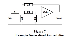



The transfer function for Figure 7 is:


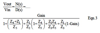
Figure 6 filter topology can implement either low-pass, high pass, or band pass characteristics by selecting R and C combinations for Z1 ,Z2, Z3, Z4, and Z5. A typical low-pass active filter configuration has; Z1=R1, Z4=R2, Z3=1/sC1, Z5=1/sC2, and Z2=open. The transfer function for this topology is shown below in Eqn 4.



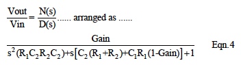
Active LP filter transfer functions arranged in the same form as Eqn. 1 and Eqn. 4 exhibit characteristics similar to passive filters. For example, the roots of D(s) are poles and the smallest pole dominates the LP cutoff frequency. In addition, the “b” coefficient of the “s” term in D(s) is the sum of the filter’s open circuit time constants (OTC) and the filter cutoff frequency is closely approximated by 1/ (2π b). Moreover, a significantly large OTC dominates the LP filter 3-dB frequency.

Active filters have an advantage over passive filters since their behavior is electronically adjustable be adjusting by the filter gain, as illustrated in Eqn. 4. For example, active filter phase angles can be tailored to fit special applications in communication and control loops.

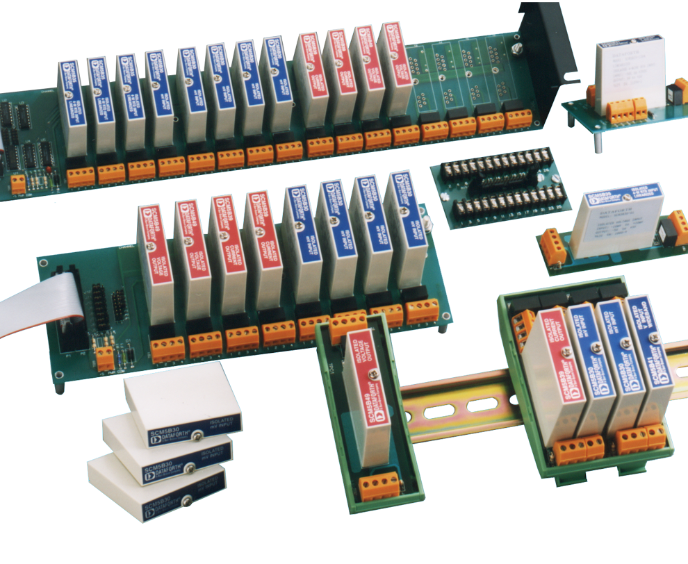
Dataforth SCM Filters

Dataforth signal conditioning products all have exacting filters incorporated in their designs. These filters are tailored to individual SCM applications. Dataforth SCMs have multi-pole low-pass filters designed for low frequency and wideband applications. Figure 8 illustrates the typical response of a Dataforth SCM 6-pole low-pass filter with a 4 Hz 3-dB frequency and a “roll-off” of 120 dB per frequency decade. Note that 50-60 Hz signals are attenuated by over 100 dB, a factor of 100,000. This represents a very effective LP filter for eliminating induced industrial noise.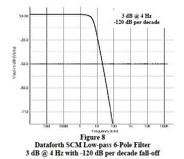



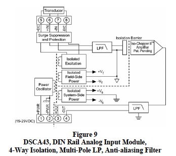
Figure 9 is the block diagram of Dataforth’s DIN-Rail signal conditioning general purpose analog input module, DSCA43. This module represents Dataforth’s 4-way isolation scheme with a multipole filter partitioned to provide anti-alaising filtering on the field side of the signal isolation barrier followed by multipole filtering on the system side of the isolation barrier. Readers are encouraged to visit Dataforth’s web site and explore their complete line of signal conditioning modules.