an121: Low Pass Filter Rise Time vs Bandwidth

Preamble

Scores of text books and hundreds of papers have been written about numerous filter topologies that have a vast spectrum of behavioral characteristics. These filters use a variety of circuit topologies made possible by today’s integrated circuits. Modern microprocessors even provide a means whereby software can be used to develop unique digital filters without analog circuitry. Clearly, it is far beyond the scope of this application note to cover all these filter topics.

The objective of this application note is to examine the low pass (LP) filter topology attributes that are common to both the leading edge rise time response to an input step voltage and the amplitude frequency response. The following bullet list represents the focus and strategy used in this Application Note.

• It is assumed that readers are familiar with the fundamental basics of circuit analysis.
• Basic circuit analysis fundamentals will be mentioned to stimulate the reader’s memory.
• Equations will be given without detail derivation.
• The examination of the LP filter’s time and frequency response will be predominately a MATLAB graphical approach (graphs are worth hundreds of words and equations) as opposed to the typical text book approach, which often analyzes filter behavior using the position of circuit poles in the left hand side of the s-plane. More on “poles” later.
• The LP filter topology of choice for analysis is the Sallen-Key Active 2-pole circuit with a passive RC section added to give an active-passive 3-pole LP filter.
• Filter analysis is limited to leading edge rise times and frequency response over the bandwidth.
• Phase analysis is not included.
• Only filters without numerator zeros will be analyzed. More on “zeros” later.

A Few Little Reminders

Filter circuit topologies contain resistors, capacitors, and inductors (modern LP filters seldom use inductors). In the early days (100+ years ago) solutions to filter circuits used differential equations since capacitor and inductor behaviors were (are) derivatives of time functions. Fortunately, numerous analytical giants have given us analytical tools for exploring circuit behavior. For example; (a) Charles Proteus Steinmetz introduced the “phasor” with complex numbers for circuit analysis. (b) Pierre Simon Laplace developed a mathematical transformation that when applied to functions of time introduces a new variable “s” that obeys simple rules of arithmetic. (c) Jean Baptiste Joseph Fourier showed that a typical time function can be expressed as a sum of individual sinusoidal terms each with their individual amplitude, frequency, and phase. (d) Leonhard Euler developed the famous exponential equation “Exp(j*x) = Cos(x) + j*Sin(x)”. Of course, we must not forget Georg Simon Ohm and Robert Gustav Kirchhoff. Without the contributions of these giants, circuit analysis in both time and frequency domains would be most difficult. The following list illustrates some reminders of R, C, and L behavior.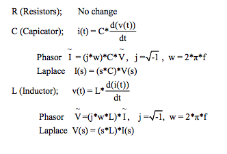



Special Reminder
The term “j” used in the above equations is the symbol commonly used in electrical engineering (other disciplines often use “i”) to represent an “imaginary number”. Now, there is nothing “imaginary” about this term, it represents an actual equation value, which is rotated 90 degrees from the x-axis (we call the x-axis the real-axis and the y-axis the imaginary-axis). The term “imaginary number” originated over a thousand years ago when early mathematicians did not know what to do with the square root of a negative number. Someone called it “imaginary” and the name stuck. Fortunately, Steinmetz and Euler showed us how to use this “j” notation in circuit analysis.

Illustrative Example

There are hundreds of LP filters circuit topologies; however, a very popular and widely used topology is the Sallen-Key circuit, shown in Figure 1. It is an active topology, very flexible, and easily manufactured thanks to the modern availability of high gain stable Op Amps (operational amplifiers). Filter response can be tailored by selected values of Rs and Cs; moreover, the amplifier gain “G” adds another powerful parameter for tailoring the filter response. In the circuit shown in Figure 1, components R4, C4, R5, C5, and the OP Amp constitute the active Sallen-Key circuit. The addition of R3, C3 adds a passive circuit contribution to the overall filter response. In these type topologies, the number of capacitors establishes the number of poles. More on “poles” later.

This type LP filter topology is a popular workhorse, which Dataforth designers use to build multi-pole filters in their SCMs. Cascading circuits as illustrated in Figure 1 will implement multi-pole LP filters. For example, cascading two circuits as shown in Figure 1 with properly chosen Rs, Cs, and Gains creates a 6-pole LP filter. Taking out one passive RC section in this cascade string, creates a 5-pole LP filter (cascading a 2-pole and a 3- pole).



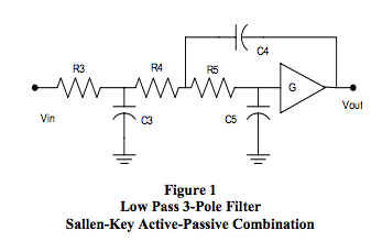
The voltage transfer function for a LP filter in Laplace notation is T(s) defined as Vout(s)/Vin(s), and is obtained by solving a set of circuit topology matrix equations using Laplace transform rules. The expression for T(s) of Figure 1 is the fraction N(s)/D(s) illustrated by Eqn. 1.



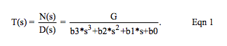
Certain circuit topologies often have factors in the numerator N(s) that cause T(s) to approach zero at some frequency. For Figure 1 topology, N(s) = G in Eqn. 1 and there are no “zeros”. As previously stated, this application note will focus on LP filter topologies with no zeros.

The matrix equations for LP filter topology in Figure 1 show that (after some messy math) the “b” coefficients in Eqn 1 are:

b3 = R3*C3*R4*C4*R5*C5
b2 = R3*C3*C5*(R4+R5) + R3*C3*C4*(1-G) ……
……. + R5*C5*C4*(R3+R4)
b1 = R3*C3 + C5*(R3+R4+R5) + C4*(R4+R3)*(1-G)
b0 = 1
Note: Terms “b2” and “b1” are functions the gain “G”

For interested circuit gurus, recall that in LP filters like this, theory shows that the “b1” coefficients are always the sum of open-circuit-time constants (OCT) as seen by each capacitor.

The basis of continued behavior analysis centers on the realization that the denominator, D(s), of the transfer function T(s) in Eqn. 1 can be factored. Recall that factoring the polynomial denominator D(s) requires one to set D(s) equal to zero and use “root” finding mathematical tools to solve for the factors (roots) w1, w2, and w3. Factoring the denominator and rearranging Eqn. 1 results in Eqn. 2.



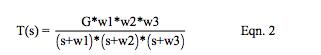
This equation format now becomes our workhorse for analyzing both the frequency and rise time responses of the LP filter in Figure 1 This effort becomes manageable with mathematical tools such as Matlab and MathCAD.

Important Note 1: If “s” in the denominator of Eqn. 2 were to mathematically equal either -w1, or, -w2, or -w3, then the denominator would go to zero and T(s) would go to infinity. This is the origin of the terminology “pole”; consequently, factors of D(s) w1, w2, w3 are called “poles” of the filter circuit, in units of radians per second.

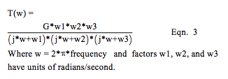
Important Note 2: In the Laplace matrix solution, the variable “s” is manipulated with simple algebraic rules. In equations such as shown in Eqn. 2 for T(s), the “frequency” response is obtained by replacing “s” with “j*w”. Thanks to the work of Laplace and Steinmetz! Frequency response T(w) is now shown in Eqn. 3.



Now, the response to a sudden step input creates the response terminology known as “rise time”, which is typically defined as the time between 10% response to 90% response of the final value (steady state output).

The rise time response examination of a LP filter provides us with information that we can not visually determine directly from the frequency response analysis even though the same circuit attributes that control frequency response control the rise time. Recall which ones? You’re correct, poles do it. Poles control both rise time and frequency responses for LP filters with no zeros.

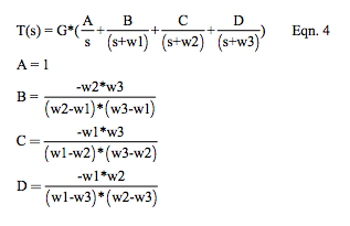
The Laplace Transform provides the best tool for deriving LP filter step responses. The Laplace equation for a unit step input is shown in Eqn. 4, which is derived from Eqn. 2 using the “Heaviside Partial Fraction Expansion” math tool.



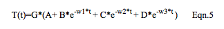
The time response to a unit step input is obtained from the rules of Inverse Laplace Transformations on Eqn. 4 with the result shown in Eqn. 5. Note: Poles do appear in the filter’s time response to a step input.

Time and Frequency Response Analysis

Before we begin a detail numerical examination, it is perhaps useful to briefly list some observations about Eqn. 3 and Eqn. 5

1. Eqn. 3 and Eqn. 5 become normalized if G = 1 after poles are calculated using actual “G” value.
2. If the frequency is zero (j*w = 0), T(w) = G
3. As the frequency approaches infinitely large values, T(w) approaches 0 at -270 degrees.
4. Given the set of w1, w2, w3, one can arrange the complex equation T(w) in Eqn. 3 as a Phasor using the rules of complex math and the works of Steinmetz. Recall a Phasor is a Magnitude with an Angle. Phasors allow us to examine filter magnitude and phase shift behavior independently as functions of frequency.

Important: The roots w1, w2, w3, of the polynomial denominator D(s) in Eqn. 2 (identified as “poles”) can be either “real” or “complex” numbers (x+j*y) or combinations of both. Recall that complex factors (poles) of D(s) always occur as complex conjugate pairs, which have identical real parts with the “j” terms differing in sign. For example, (3+j*4) and (3-j*4) are complex conjugate pairs. We will see later that complex poles introduced into Eqn. 3 and Eqn. 5 are responsible for ringing overshoots in the filter’s leading edge time response and peaking in the filter’s frequency response.

The magnitude of Eqn.3 is often plotted in different graphical environments using different axis scales, which can emphasize or suppress certain filter performance characteristics. See Figure 2.c.

Table 1 shows the component values used for Figures 2 and 3 behavior plots of the Sallen-Key circuit in Figure 1.



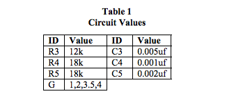
The plots in Figure 2 were generated by a Matlab program for the 3-Pole LP Filter Topology shown in Figure 1 with component values from Table 1. This Matlab program changes the Op Amp gain “G” which changes the roots (poles) of D(s) because coefficients “b2” and “b1” in Eqn. 1 are functions of “G”. These gain changes tailor the LP filter time and frequency response data. Plots are normalized. Showing all normalized response plots together allows a single graphical view to illustrate how different poles influence filter responses and how different frequency axis scale factors enhance or compress behavioral traits. Bandwidth, Rise Time, and Pole data are shown below in Table 2.





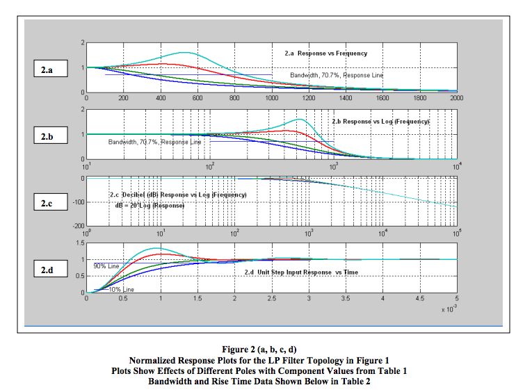
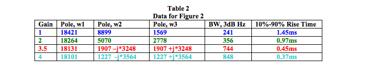
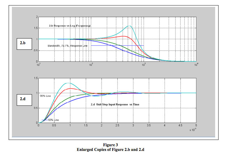
Figure 3 is an enlarged copy of Figure 2.b and 2.d for enhanced viewing.

Important Observations about Low Pass Filter Responses without N(s) Zeros

The examination of Table 2, Figures 2, and 3, illustrate some significant facts about LP filter responses as follows;

• Low pass filter specifications must be viewed in both time and frequency perspectives.
• Real poles do not cause a peak in the frequency response (frequency peaking).
• Real poles do not cause overshooting and ringing in the leading edge time (rise time) response.
• Certain combinations of real poles can increase bandwidth and decrease rise time.
• Complex poles can cause frequency peaking in the bandwidth region.
• Complex poles can cause ringing (over and under shoots) in the leading edge response to a unit step input.
• Complex poles can cause significant increase in bandwidth and significant decrease in rise time.
• he same leading edge rise time “ringing” issues occur on the response fall time, not shown here.
• When a LP filter’ rise time (and fall time) rings, the settling time is an issue in addition to the amounts of over/under shoots. Note: Settling time is determined by how long it takes for the exponential terms “Exp(-k*t)” in Eqn. 5 to decay to zero. Mathematically this requires the time “t” to become infinitely large; therefore, settling time must be specified as an acceptable % of the LP Filter’s final (steady state) response value to a unit step input.
• Figure 2.c illustrates the frequency response of a LP Filter plotted in dB [dB = 20*Log(normalized frequency response)] on the y-axis scale vs the Log(frequency) on the x-axis. This type plot has two important features;
  a. Creates a visual illusion by suppressing frequency peaking and presents frequency response as almost flat.
  b. Shows that the frequency attenuation beyond the bandwidth frequency approaches an attenuation equal to the (number of LP filter poles) *(20) in units of dB per decade change in frequency. For example, a 3-pole filter falls at 60dB (1E-3) per decade and a Dataforth 7-pole filter falls at 140 dB (1E-7) per decade, which is far more effective at suppressing unwanted frequencies. See Figure 4.

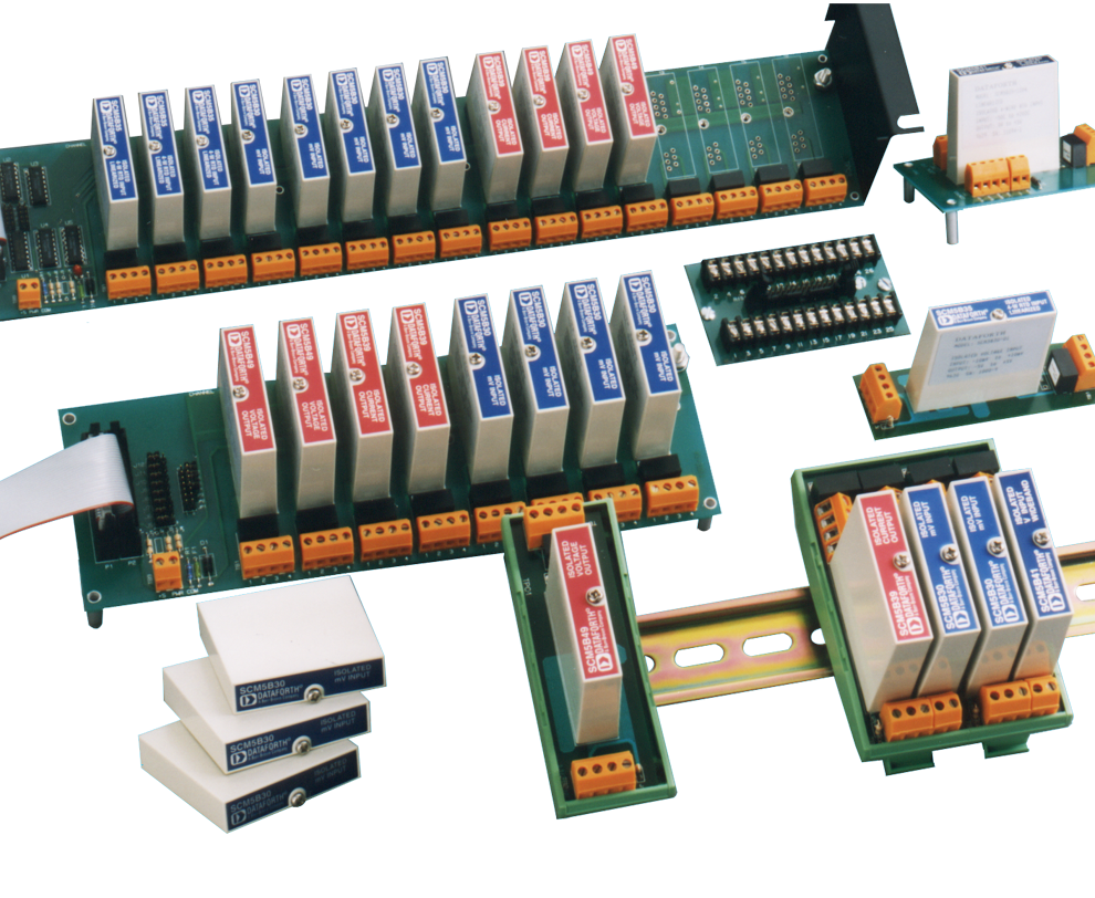
Dataforth Signal Conditioning Module (SCM) Low Pass Filter

Figure 4 represents a Dataforth SCM generic 7-pole LP filter frequency and unit step response. Dataforth designers are professionals with decades of experience in filter design. They balance the attributes of selected poles in multi-pole filter topologies to provide near ideal low pass filter behavior. Moreover, Dataforth realizes that industrial data acquisition and control systems must have premium high quality filters for noise suppression and aliasing prevention. Figure 4 visually illustrates some outstanding attributes of quality multi-pole low pass filtering that Dataforth designs in all their SCMs. These are the qualities necessary for premium low pass filtering in SCMs. Readers are encouraged to visit Dataforth’s website and examine Dataforth’s complete line of SCM filter attributes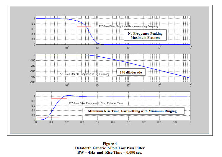

Rise Time vs Bandwidth

Remember the works of Jean Baptiste Joseph Fourier who showed that a function of time could be represented by an infinite sum of individual sinusoidal functions, each with their individual amplitudes, frequency, and phase shift. Consider the unit step function of time with an almost zero rise time (certainly almost infinitely fast). In order to represent this leading edge with a sum of individual sinusoids (via Fourier) would require a large collection of very high frequency sinusoids.

Low Pass Filters embedded as an integral part of any premium quality SCM has a bandwidth frequency beyond which high frequencies are steeply attenuated. Now this means that the bandwidth of a SCM limits the LP filter rise time. Therefore, one would naturally assume that knowing the bandwidth, one should be able to determine the 10%-90% rise time.

A simple unique closed form equation that derives the rise time of a multi-pole LP filter given only the filter’s bandwidth is beyond practicability. However, there is a way to get a prediction (operative word here is prediction) of LP filter rise time given bandwidth.

A single RC low pass filter has a 10%-90% rise time equation of [Rise Time = 0.35/ (BW, Hz)], which says rise time is inversely proportion to bandwidth. Does this expression work for LP filters with multiple poles some of which are complex?



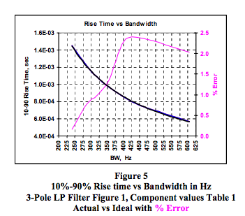
Figure 5 shows a comparison between actual results for the 3-pole LP filter of Figure 1 and an ideal single pole RC LP filter. Results give less than a 2.5% error.

Conclusion from Figure 5
Assuming a reasonably well behaved multi-pole LP filter, one can predict (make a reasonable estimate on) the filter’s 10%-90% rise time given the filter’s frequency bandwidth by using [Rise Time = 0.35/ (BW, Hz)] . Using this estimate on the Dataforth 7-pole generic LP filter in Figure 4 gives a rise time of 0.0875 sec. where actual is 0.090 sec. This relationship only gives a prediction, which is close; nevertheless, use it with caution.

Final Note

To completely understand the complete characteristics of LP filters requires one to examine filter response specifications attributes from two different perspectives, both “time” and “frequency”. This examination should look at both time and frequency behavior traits necessary for the user’s specific applications.

The reader is encouraged to visit Dataforth’s web site and explore their complete line of isolated signal conditioning modules and related application notes, see the reference shown below.

Dataforth References

1. Dataforth Corp.,
http://www.dataforth.com