an107: Practical Thermocouple Temperature Measurements

Preamble

The theory of thermocouple behavior is discussed in Dataforth's Application Note AN106, Introduction to Thermocouples. The reader is encouraged to examine this Application Note for thermocouple background and fundamentals. For additional details on thermocouple interface products the reader should visit this website's offering on Thermocouple Signal Conditioning.

There is an abundance of additional information available on thermocouples from various sources. The interested reader is encouraged to visit those references listed at the end of this Application Note.

Thermocouple Types

Thermocouples have become standard in the industry as a cost effective method for measuring temperature. Since their discovery by Thomas Johann Seebeck in 1821, the thermo electrical properties of many different materials have been examined for use as thermocouples. The standards community together with modern metallurgy has developed special material pairs specifically for use as thermocouples.

Table 1 displays industries eight popular standard thermocouples and their typical attributes. The letter type identifies a specific temperature-voltage relationship, not a particular chemical composition. Manufacturers may fabricate thermocouples of a given type with variations in composition; however, the resultant temperature versus voltage relationships must conform to the thermoelectric voltage standards associated with the particular thermocouple type.

Complete sets of temperature versus voltage tables referenced to zero °C and including mathematical models for all popular industry standard thermocouples are available at NIST, the National Institute of Standards and Testing, and can be downloaded free of charge from their web site, Reference 1. The reader is encouraged to examine this website for additional information..

Table 1: Standard Thermocouple Types


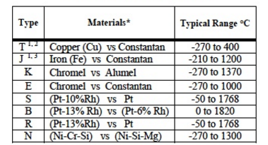
* Material Definitions:

• Constantan, alloy of Nickel (Ni) - Copper (Cu)
• Chromel, alloy of Nickel (Ni) - Chromium (Cr)
• Alumel, alloy of Nickel (Ni) and Aluminum (Al)
• Magnesium (Mg), base element
• Platinum (Pt), base element
• Nickel (Ni) a base element
• Silicon (Si), a base element
• Chromium (Cr), a base element
• Iron (Fe), a base element
• Rhodium (Rh), a base element

Notes:

1. Both the L and U Type thermocouples are defined by DIN Standard 43710; however, they are not as frequently used in new installations as the more popular T and J Type thermocouple standards.
2. The U Type thermocouple is similar to the popular standard T Type
3. The L Type thermocouple is similar to the popular standard J Type

Three additional thermocouple types used for high temperature measurements are C, D, and G Type thermocouples. Their designation letters (C, D, G) are not recognized as standards by ANSI; nonetheless, they are available. Their wire compositions are;

• G Type: W vs W-26%Re
• C Type W-5%Re vs W-26%Re
• D Type W-5%Re vs W-25%Re

Where; "W" is Tungsten and "Re" is Rhenium

Most all practical temperature ranges can be measured using thermocouples; even though, their output full-scale voltage is only millivolts with sensitivities in the microvolts per degree range and their response is non-linear. Figures 3 and 4 at the end of this Application Note displays typical voltage-temperature characteristics of the above thermocouples. These curves provide a visual indication of thermocouple ranges, scale factors, sensitivities, and linearity

Dataforth offers thermocouple input modules, which interface to all the above types. For more details on these and other state-of-the-art modules, visit Dataforths website, Reference 2.

The Thermocouple Analytical Model

Standard mathematical power series models have been developed for each type of thermocouple. These power series models use unique sets of coefficients which are different for different temperature segments within a given thermocouple type. Unless otherwise indicated, all standard thermocouple models and tables are referenced to zero degrees Centigrade, 0°C. The reader is referred to Dataforths Application Note AN106, Introduction to Thermocouples for the fundamentals of thermocouples, Reference 8.

Reference for the following examples and associated data is the NIST, National Institute of Standards and Testing; website, Reference 1. Equation 1 illustrates the power series model used for all thermocouples except K Type, which is illustrated by Eqn. 3


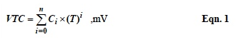
Where T is in degrees C

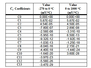
The set of coefficients used in Eqn. 1 to model E Type thermocouple is shown for 3 significant digits in Table 2.

Table 2: Coefficients C_i for Type E Thermocouple


These equations with their different sets of coefficients are difficult to use in directly determining actual temperatures when only a measured thermocouple voltage [VTC] is known. Therefore, inverse models have been developed to determine temperatures from measured thermocouple voltages. Equation 2 represents this inverse model.


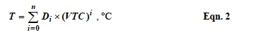
Where VTC is in millivolts

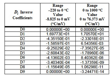
The sample set of inverse coefficients for E Type thermocouples is shown for 6 significant digits in Table 3.

Table 3: Inverse Coefficients for E Type Thermocouple

It is noteworthy to mention here that K Type V1 = S*(Tx-Tc) Eqn. 4 thermocouples require a slightly different power series model. Equation 3 represents the standard mathematical power series model for Type K thermocouples.



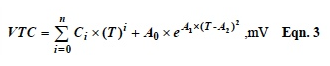
The exponential term 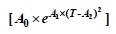in Eqn. 3 is added to account for special effects. More details on this type thermocouple model are available from NIST web site, Reference 1.

Cold Junction Compensation (CJC) Technique

Standard thermocouple look-up tables and models are referenced to zero °C; whereas, field measurement topologies are made with the thermocouple connected to a connector that is not at zero °C; consequently, the actual measured voltage must be adjusted so that it appears as referenced to zero °C.

Modern signal conditioning modules have electronically resolved this situation and, in addition, have linearized the thermocouple voltages. These conditioning modules provide the end-user with a linear output signal, scaled to either volts per °C (°F) or amps per °C (°F). The concept of electronically referencing thermocouple measurements to zero °C is shown in Figure 1. This technique is known as ìcold junction compensationî or CJC.


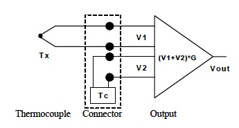
Figure 1: Cold Junction Compensation Concept

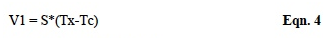
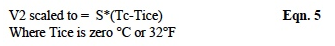
In Figure 1, the voltage V1 is Seebeckís thermocouple voltage generated by the difference between the unknown temperature (Tx) and the connector temperature (Tc), as shown in Equation 4. The connector temperature (Tc) is measured with a non-thermocouple sensor (diode, RTD, etc.) and the corresponding sensor voltage (V2) is electronically scaled to represent the same Seebeck thermocouple voltage (referenced to 0°C) that a thermocouple would read if used to measure Tc as indicated in Eqn. 5. This ìV2 scalingî is matched to the same type thermocouple as used to measure Tx.



The reader is referred to Reference 8, Dataforthís Application Note AN106 for the derivation of these expressions.

Equation 4 can be mathematically rearranged to include the ice-point temperature (Tice).



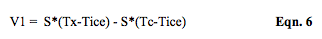
Equation 6 shows the thermocouple voltage (V1) has two parts, both of which are referenced to Tice. The voltage term, S*(Tx-Tice), is the standard look-up table value needed for determining the unknown temperature (Tx). The term, S*(Tc-Tice), is the voltage obtained if connector temperature (Tc) were measured with the same type thermocouple as used to measure Tx. Recall that V2 has been electronically scaled so that V2 equals this voltage, V2 = S*(Tc-Tice). In Figure 1 if G = 1, then;



The output voltage (Vout) in Equation 7 can be entered directly into the appropriate type thermocouple reference table to determine the measured temperature.

Linearization

Accurate thermocouple measurements need signal conditioning modules with outputs, which are linearly scaled to temperature. Module output voltages which have linear scale factors in volts per degree or amps per degree eliminate the need for look-up tables or power series expansions since the conversion from thermocouple volts to temperature is built into the linearized output scale factor. Such thermocouple signal conditioning modules including isolation and CJC are available from Dataforth.

Figure 3 displays the voltageñtemperature curves for eight of the most common thermocouples. These curves are presented here to show a visual indication of standard thermocouple ranges, magnitudes of output voltages, nonlinearity and sensitivity (mV/°C). Although the operational temperature ranges over which thermocouples can be used is quite large, their sensitivity is small; in the microvolt per °C range. In addition, Figure 3 illustrates that for negative temperatures, thermocouplesí response is very non-linear; however, these curves appear near linear for certain ranges of positive temperatures. Nonetheless, the fact remains that thermocouples are non-linear.

As an example of non-linearity, Figure 2 illustrates thermocouple non-linearity by plotting the difference between an ideal linear response and the response of a Type J thermocouple over the range of 0 to 150 °C.


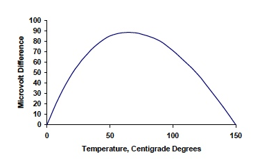
Figure 2: Output Voltage Difference Between Ideal Linear Sensor and J Type Thermocouple

The sensitivity of a J Type thermocouple is approximately 54 µV/ °C. It is obvious from Figure 2 that assuming a linear response for J Type thermocouples could result in nearly two degrees of error.

Clearly, linearization is necessary to facilitate accurate temperature measurements with thermocouples. Dataforth has developed proprietary circuit techniques, which provide precise linearization for their signal conditioning modules. Although modern PCs or other embedded microprocessors can linearize thermocouples using software techniques, hardware linearization provides faster results and does not burden valuable computer resources.

To achieve linearity, the gain (G) in Figure 1 and Equation 7 is internally programmed to selectively scale the voltage function S*(Tx-Tice) to be a linear function of temperature with the units of volts per °C (°F) or milliamps per °C (°F). For more details, examine AN505 ìHardware Linearization of Non-linear Signalsî on Dataforthís website application note section, Reference 9. While on this web site, take a few moments to examine all of Dataforthís complete line of thermocouple signal conditioning modules.

Figure 5 of this Application shows a functional blockdiagram with typical specifications of a Dataforth thermocouple signal-conditioning module.

Practical Considerations

The following is a list of some "mind joggers" for consideration when measuring temperature with thermocouples.

1. Always examine thermocouple manufacturers specifications for conformity to standards, specified temperature ranges, and interchangeability.


2. Reproducibility and interchangeability between brands of thermocouple should be examined. Errors due to thermocouple replacement should be avoided.


3. Use isolated signal conditioning modules to avoid ground loops.


4. Always use thermocouple signal conditioning modules with appropriate input filtering. This could avoid serious ìnoiseî errors.


5. Each thermocouple wire connected to the sensing module must be at the same temperature. Module connectors should have no thermal gradients across the individual connections.


6. Thermocouple behavior depends on the materialsí molecular structure. Environmental conditions such as stress, chemical corrosion, radiation, etc that affect molecular structure anywhere along the length of the thermocouple wire can create errors. For example, thermocouples with iron composition are subject to rust, which can cause errors.


7. Use twisted pair extension wires and signal conditioning modules with adequate filtering to help avoid EMI and RFI errors.


8. Keep thermocouple lead lengths short.


9. Use manufacturerís recommended extension wires if long thermocouple leads are necessary.


10. Always observe color code polarity. Note: Some European manufacturers use the opposite color for positive and negative polarity than North American manufacturers.


11. Avoid ìheat shuntsî when installing thermocouples. Any heat conducting material, like large lead wires, may shunt heat away from the thermocouple, creating an error


12. Hostile corrosive environments combined with moisture and heat may cause corrosion, which can stimulate galvanic action and create electrochemical voltage errors.


13. Recall that temperature measurement response time is significantly impacted by the thermocouple package encapsulation. For example, thermocouples in a ìthermal wellî have a slow response time, which may cause undesirable hunting in a control loop.


14. Thermocouple enclosures are available with thermocouples connected to the enclosure. These are ìgrounded thermocouplesî and may cause ground loop problems. Considering using isolated modules to avoid such problems.


15. Ensure that signal conditioning modules with electronic CJC techniques use temperature-sensing devices, which have thermal response times equivalent to that of the measurement thermocouples.

Figure 3 illustrates the spectrum of voltage-temperature characteristics of the most popular standard thermocouples


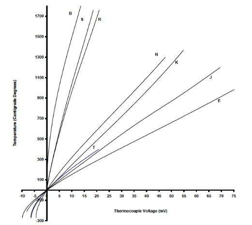
Figure 3: Voltage-Temperature Characteristics of B, E, J, K, N, R, S, and T Type Thermocouples

Figure 4 illustrates the spectrum of voltage-temperature characteristics of high temperature thermocouples, which are not classified by ANSI.


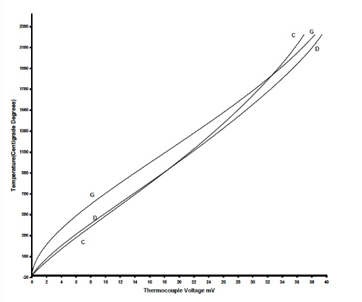
Figure 4: Voltage-Temperature Characteristics of G, D, C Type Thermocouples

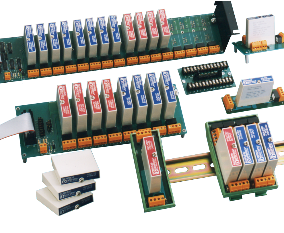
Figure 5 illustrates an example of Dataforth's SCM5B47 Isolated Linearized Thermocouple module. Dataforth offers a complete line of modules for all thermocouple types. Theses modules offer excellent isolation, superior accuracy and linearity. See Dataforthís website http://www.dataforth.com.



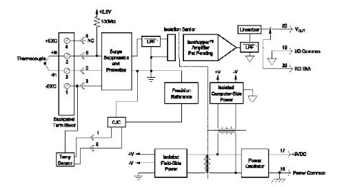
Figure 5: Dataforth's SCM5B47 Isolated Linearized Thermocouple Module

Each SCM5B47 thermocouple input module provides a single channel of thermocouple input which is filtered, isolated, amplified, linearized and converted to a high level analog voltage output (Figure 5). This voltage output is logic-switch controlled, allowing these modules to share a common analog bus without the requirement of external multiplexes.

The SCM5B modules are designed with a completely isolated computer side circuit, which can be floated to ±50V from Power Common, pin 16. This complete isolation means that no connection is required between I/O Common and Power Common for proper operation of the output switch. If desired, the output switch can be turned on continuously by simply connecting pin 22, the Read-Enable pin, to I/O Common, pin 19.

The SCM5B47 can interface to eight industry standard thermocouple types: J, K, T, E, R, S, N, and B. Its corresponding output signal operates over a 0V to +5V range. Each module is cold-junction compensated to correct for parasitic thermocouples formed by the thermocouple wire and screw terminals on the mounting backpanel. Upscale open thermocouple detect is provided by an internal pull-up resistor. Downscale indication can be implemented by installing an external 47MW resistor, ±20% tolerance, between screw terminals 1 and 3 on the SCMPB01/02/03/04/05/06/07 backpanels.

Signal filtering is accomplished with a six-pole filter, which provides 95dB of normal-mode-rejection at 60Hz and 90dB at 50Hz. Two poles of this filter are on the field side of the isolation barrier, and the other four are on the computer side.

After the initial field-side filtering, the input signal is chopped by a proprietary chopper circuit. Isolation is provided by transformer coupling, again using a proprietary technique to suppress transmission of common mode spikes or surges. The module is powered from +5VDC, ±5%.

A special input circuit on the SCM5B47 modules provides protection against accidental connection of power-line voltages up to 240VAC.

References

1. NIST, National Institute of Standards and Testing
2. Dataforth Corp.
3. Rosemount
4. Omega
   a. http://www.omega.com/temperature/Z/zsection.asp
   b. http://www.omega.com/temperature/Z/pdf/z246.pdf
5. ASTM, American Society for Testing and Materials
6. IEC, International Electrotechnical Commission
7. ANSI, American National Standards Institute
8. Dataforth Application Note AN106, Introduction to Thermocouples
9. Dataforth Application Note AN505, Hardware Linearization of Non-linear Signals

Standards Related to Thermocouples

• DIN 43722
• DIN 43714
• DIN 43760
• DIN 43710
• IEC 304
• IEC 751
• DIN IEC 548
• ANSI MC 96-1-82
• JIS C 1602-1981