

an124: Tuning Control Loops with the IMC Tuning Method
Application Note
Preamble
Since 1942, well over one hundred controller tuning methods have been developed, each trying to accomplish a certain objective or fill a specific niche. One of these methods is the Internal Model Control (IMC) tuning method [Ref. 2], sometimes called Lambda tuning. It offers a stable and robust alternative to other techniques, such as the famous Ziegler-Nichols method, that usually aim for speed at the expense of stability. This Application Note describes how to tune control loops using IMC tuning rules.Applicable Process Types
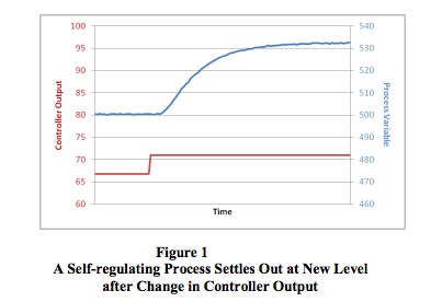
The IMC tuning method was developed for use on selfregulating processes. Most control loops, e.g., flow, temperature, pressure, speed, and composition, contain self-regulating processes. One obvious exception is a level control loop, which contains an integrating process.A self-regulating process always stabilizes at some point of equilibrium, which depends on the process design and the controller output. If the controller output is set to a different value, the process will respond and stabilize at a new point of equilibrium (Figure 1).
Advantages and Disadvantages of IMC Tuning
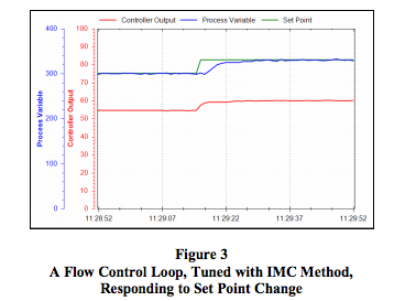
The IMC tuning method offers the following advantages:- Once tuned using the IMC tuning rules, the process variable will not overshoot its set point after a set point change.
- The IMC tuning rules are much less sensitive to possible errors made when determining the process dead time through step tests. It is easy to under- or over-estimate dead time on lagdominant processes because of their relatively short dead times. Ziegler-Nichols and many other tuning rules can give poor results when the dead time is measured incorrectly.
- The tuning is very robust, meaning that the control loop will remain stable even if the process characteristics change substantially from the ones used for tuning.
- An IMC-tuned control loop absorbs disturbances better and passes less of them on to the rest of the process. This is a very attractive characteristic for using IMC tuning in highly interactive processes.
- The user can specify the desired control loop response time (the closed-loop time constant). This provides a single “tuning factor” that can be used to speed up and slow down the loop response.
Unfortunately, the IMC tuning method has a drawback, too. It sets the controller’s integral time equal to the process time constant. If a process has a very long time constant, the controller will consequently have a very long integral time. Long integral times make recovery from process disturbances very slow.
Target Controller Algorithm
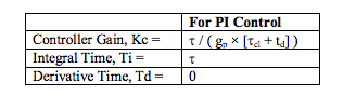
The IMC tuning rules are designed for use on a noninteractive controller algorithm. The tuning rules presented here are for a PI controller. Although IMC tuning rules have also been developed for PID controllers, there is theoretically no difference in the speed of response of the PI and PID tuning rules, so there is little sense in adding the complexity of derivative control.Procedure
- Do a step test:
- Put the controller in manual and wait for the process to settle out
- Make a step change in the controller output (CO) of a few percent and wait for the process variable (PV) to settle out. The size of this step should be large enough that the PV moves well clear of the process noise/disturbance level. A total movement of five times more than the peak-to-peak level of the noise and disturbances on the PV should be sufficient.
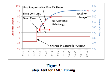
- Determine the process characteristics (refer to Figure 2):
- If the PV is not ranged 0-100%, convert the
change in PV to a percentage of the range as
follows:
Change in PV [in %] = change in PV [in Eng. Units] × 100 / (PV upper calibration limit - PV lower calibration limit) - Calculate the Process Gain (gp):
gp = total change in PV [in %] / change in CO [in %] - Find the maximum slope of the PV response curve. This will be at the point of inflection. Draw a tangential line through the PV response curve at this point.
- Extend this line to intersect with the original level of the PV before the step in CO.
- Take note of the time value at this intersection
and calculate the Dead Time (td):
td = time difference between the change in CO and the intersection of the tangential line and the original PV level - If td was measured in seconds, divide it by 60 to convert it to minutes. Since the Dataforth PID controller uses minutes as its time base for integral time, all measurements have to be made in minutes.
- Calculate the value of the PV at 63% of its total change.
- On the PV reaction curve, find the time value at which the PV reaches this level.
- Calculate the Time Constant (τ):
τ = time difference between intersection at the end of dead time, and the PV reaching 63% of its total change - If τ was measured in seconds, divide it by 60 to convert it to minutes.
- Repeat steps 1 and 2 three more times to obtain good average values for the process characteristics.
- Choose a desired loop response time (closed loop time constant, τcl) for the control loop. Generally, the value for τcl should be set between one and three times the value of τ. Use τcl = 3 × for a very stable control loop. Using a larger value for τcl will result in a slower control loop, while using a smaller value will result in a faster control loop.
- Calculate PID controller settings using the equations below.
- Enter the values into the controller, make sure the algorithm is set to Noninteractive, and put the controller in automatic mode.
- Change the set point to test the new values.
- Do fine tuning if necessary. The control loop’s response can be sped up by increasing Kc and/or decreasing Ti.
Conclusion
While many PID controller tuning rules aim for a fast response but sacrifice loop stability to obtain that fast response, the IMC tuning rules provide a viable alternative when control loop stability is important.References
[1] J.G. Ziegler and N.B. Nichols, Optimum settings for automatic controllers, Transactions of the ASME, 64, pp. 759–768, 1942[2] D.E. Rivera, M. Morari, and S. Skogestad, Internal Model Control. 4. PID Controller Design, Industrial Engineering and Chemical Process Design and Development, 25, p. 252, 1986
The reader is encouraged to visit Dataforth’s website to learn more about PID control and the MAQ® 20.
- Application Note 122: Introduction to PID Control
http://www.dataforth.com/catalog/pdf/AN122.pdf - MAQ® 20 Brochure
http://www.dataforth.com/catalog/pdf/MAQ20_broch ure.pdf
Was this content helpful?
Thank you for your feedback!