an116: Why Use Isolated Signal Conditioners?

Preamble

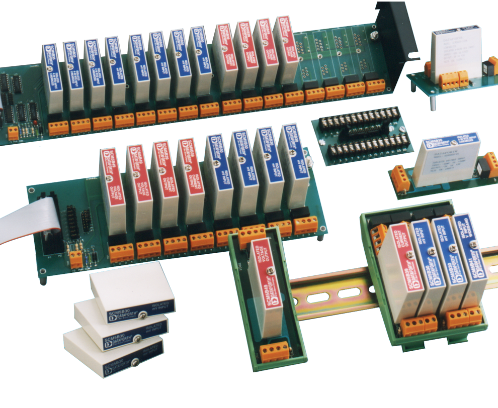
Isolating power sources and sensor signals is the most effective method for eliminating undesirable ground loop currents and induced electrical noise. Dataforth Signal Conditioning Modules (SCMs) use up to four levels of isolation to eliminate ground loop problems and induced field noise. The reader is encouraged to visit Dataforth’s website and examine the complete line of isolated SCMs. For additional reading on isolating unwanted ground loop currents, see Reference 2.

Answer Five PC-Based Measurement Questions with Isolated Signal Conditioners

When you move a data acquisition system from the controlled environment of the laboratory to validation testing or the manufacturing floor, some problems may arise. Many factors may combine to destroy measurement accuracy, or possibly even the equipment. Understanding these factors is crucial to measurement success.

Five recurring roadblocks to successful measurements are addressed here, in the order of most to least common, together with some real-life examples. This discussion will provide an understanding of how measurement inputs become corrupted and the need to isolate them.

1. Crosstalk
By far the most common question heard involves a phenomenon where the contents of one data acquisition channel are superimposed on another. This condition, known as crosstalk, can cause subtle to major measurement errors that may go undetected. In its most exaggerated form, a nearly exact duplicate of one channel appears on an adjacent channel to which nothing is connected.

The PC-based instrumentation revolution generated active use of multiplexers. The revolution is driven by the promise of low cost per channel, with a target per-channel cost of $30 to $40. However, along the way, the hallmark of traditional instrumentation has been dropped – an isolation amplifier for each channel. The system-undertest is connected directly to the multiplexer's inputs; however, the multiplexer is not an ideal signal processing device. Its inputs have capacitance that stores a charge that is directly proportional in magnitude to the sample rate and the impedance of the signal source. This inherent characteristic causes crosstalk.

Consider an application where the multiplexer’s input is connected directly to the output of an isolation amplifier. In this situation, the impedance the multiplexer sees is stable and low, with 10Ω being a typical value. Crosstalk is greatly minimized, or eliminated altogether, since the impedance of the source is low enough to bleed off the charge on the multiplexer's input capacitance before the analog-to-digital converter (ADC) reports a value.

Even under this nearly ideal impedance situation, a high sample rate can boost crosstalk by minimizing the capacitive discharge time on the multiplexer's channels. In effect, the capacitance has less time to bleed off its charge before the analog-to-digital conversion takes place, resulting in crosstalk where none existed before.

As source impedance and sample rate increase, the probability of crosstalk increases as well. To prevent this from happening, keep these points in mind:

• Minimize the source impedance of the signal source. Use isolation amplifiers to keep it below 100Ω , although at very high sample rates, even this value may be too high.


• When source impedance cannot be controlled, an isolation amplifier is needed between the signal source and the data acquisition card multiplexer. An instrument with a built-in isolation amplifier is needed on each channel to provide protection from stray signal paths.


• These strategies become even more important as the sample rate increases. The best and most predictable results are obtained when an instrument is used that has a fixed scan interval; this helps control any high sample rate bursts.

2. Common-Mode Voltage
Although crosstalk leads the list in number of measurement problems, common-mode voltage (CMV) leads in its capability to distort data.

Using familiar measurement methods, like a batterypowered, hand-held digital voltmeter (DVM), input readings are almost impervious to CMV problems. Many engineers assume they can extend the success of DVMs to PC-based measurement approaches. However, in most cases, the results range from poor to disastrous.

The problems encountered are tied to two specifications on the manufacturer's data sheet: full-scale input range and maximum input voltage (without damage). Full-scale input range indicates the magnitude of voltage connected across the instrument's inputs (normal-mode voltage or NMV), which can successfully be measured. As its name implies, maximum input voltage indicates how much NMV the instrument will tolerate before incurring damage.

The CMV, which appears simultaneously and in phase on each of the instrument's inputs with respect to power ground, combines with the NMV to test the limits of the measurement system. Most data acquisition products for the PC permit measurements when the sum of CMV and NMV is equal to or less than the instrument's full-scale input range.

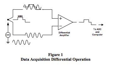
Measurements can be made under these conditions only if the data acquisition product’s input is configured for differential operation as shown in Figure 1. With this basic rule for differential measurements established, here are the possible measurement results, in the order of best to worst:

• (CMV + NMV) ≤ Full Scale Range: This is a good measurement, subject to the common-mode rejection (CMR) specification of the instrument.


• Full Scale Range ≤ (CMV + NMV) ≤ Maximum Input Voltage (without damage): The measurement could be latched at plus or minus, full scale. There are no usable measurement results, but no damage either.



• (CMV + NMV) > Maximum Input Voltage (without damage): There is potential for damage to the data acquisition product and to the attached computer.

For most data acquisition products, it doesn't take long to reach the destructive stage. Most will tolerate a maximum input voltage (without damage) of ±30VDC or peak AC. In the realm of production measurements, with 120V to 440VAC motor supplies or 24VDC process current supplies and the high probability of ground loops, this limit can be very quickly and irrevocably exceeded.



How can the comparatively expensive data acquisition instrument be used to collect the same measurements that are made so effortlessly and safely with the hand-held DVM? The answer is to choose a product that provides isolation.

Isolation is what its name implies. As with a batterypowered DVM, there is no electrical connection between the common connection associated with the instrument's front-end input terminals and the power common connection associated with the back-end of the instrument and the computer.

As such, the instrument's front end is free to float at a level defined by the magnitude of the CMV, without damage and with complete measurement accuracy. Here, the maximum CMV that can be tolerated is not dictated by its maximum input voltage specification, or even by its full-scale range, but rather by the voltage at which the isolation barrier breaks down.

For example, with most Dataforth isolated signal conditioning products, isolation barrier breakdown occurs above 1500VAC or 2200VDC, which is much higher than the expected CMV of most production applications.



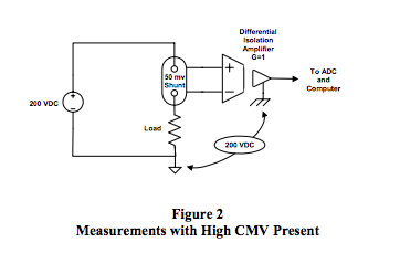
Figure 2 describes a typical application where isolation allows a measurement in the presence of a high CMV.

Understand that isolation can be provided in more than one form: input-to-output, channel-to-channel, and a combination of both. For the vast majority of multichannel production applications, both input-to-output and channel-to-channel isolation are needed. Such an arrangement allows each channel’s input to float with respect to all other channels.

A CMV on channel one, for example, will not disrupt measurements on the other channels, even if they are referenced to power supply ground, the same CMV, or an entirely different CMV. In contrast, systems designed with just input-to-output isolation essentially tie together the CMVs of all the channels. A CMV on one channel floats all channels at the same voltage with potentially disastrous results if another channel is connected to a ground-referenced signal or a different CMV.

There is only one reason to buy a product that offers only input-to-output isolation, and that reason is cost. For example, it is less expensive to build one isolation barrier into an 8-channel product than one for each channel. The cost savings usually are reflected in a lower system price. However, in the actual application of such an instrument, the initial cost savings may be offset by expensive repairs later.

Before leaving the topic of isolation, one point needs to be established firmly and clearly: Do not confuse a product that offers differential measurement capability with one that offers isolation. These are two entirely different and unrelated features.

Moreover, some engineers are still under the impression that a product with differential measurement capability allows them to apply the instrument in high CMV conditions. As discussed previously, differential but nonisolated inputs tolerate only moderate CMVs (without damage) and even lower CMVs are required for more trustworthy measurement results.

3. DC Common-Mode Rejection (CMR)
Whenever a measurement is made in the presence of a CMV, accuracy will be adversely affected. The question that remains is the magnitude of the inaccuracy. This can be determined by looking up the specification for CMR in the product's data sheet. Any instrument that provides a differential input, isolated or not, offers the capability to reject a CMV to a degree determined by its CMR. CMR is most commonly defined as a logarithmic ratio of input-tooutput CMV (in decibels). The common-mode rejection ratio (CMRR) for most general purpose, analog-to-digital products for the PC is around 80dB. How does this figure apply to the measurement? Here’s a simple example that includes the math.

Example 1
Assume that you want to measure a 3VDC normal-mode signal in the presence of a +6VDC CMV, and assume that the normal-mode signal gain is 1.

• 80dB = 20 log (VCMV in / VCMV out)


• 80dB = 20 log (6VDC / VCMV out)


• 4 = log (6VDC / VCMV out)


• 10,000 = 6VDC / VCMV out


• VCMV out = 0.6mV

Measurement Accuracy = 3VDC +0.6mV, or +0.02%

The measurement accuracy determined in the example above would be considered reasonable for most applications. The starting CMV was twice the magnitude of the starting signal. The differential amplifier, with its 80dB CMRR specification, reduced the CMV’s effect on the amplifier's output to fractions of a millivolt, with a negligible impact on accuracy. It may appear from this example that 80dB rejection is suitable for most applications.

Example 2
The following example tests that hypothesis, using the real-world application shown in Figure 2.

• 80dB = 10,000 = +200VDC / VCMV out


• VCMV out = +20mV

Measurement Accuracy = 50mV +20mV, or +40%

The instrument that works well when the spread between the CMV and NMV potentials is narrow (only 2:1 in the first example) fails when the spread increases exponentially. This is a common situation in many production measurements, like the 4,000:1 spread of the typical current shunt measurement in Figure 2.



Since you cannot lower the CMV in these situations, the only solution is to apply an instrument with better CMR.

Example 3
Here's how the math stacks up for the same application using 120dB CMRR:

• 120dB = 20 log (VCMV in / VCMV out)


• 120dB = 20 log (200VDC / VCMV out)


• 6 = log (+200VDC / VCMV out)


• 1,000,000 = (+200VDC / VCMV out)


• VCMV out = +0.2mV

Measurement Accuracy = 50mV +0.2mV, or +0.4%

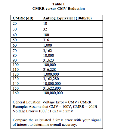
As the examples show, knowing how a CMV will affect measurement accuracy is at least as important as knowing that it exists. To help evaluate an instrument you may already have or might purchase, Table 1 provides a guide to the error caused by a CMV as a function of your instrument's CMRR.

To use it, determine the CMV of the application and look up the instrument's CMRR specification on its data sheet.

Table 1 provides a range of CMRRs in decibels and their equivalent antilog ratios, making it unnecessary to work with logarithmic math.

Plug the appropriate CMV and antilog ratio into the equation shown. The result is the expected measurement error in volts. To determine the instrument's suitability for the application, compare the resulting figure with the NMV you need to measure.

4. AC Common-Mode Rejection (CMR)
AC CMVs are as prevalent as DC CMVs, and even more so when you include unpredictable noise sources such as motor brushes and inductive conducted and radiated electromagnetic fields (EMFs). Therefore, the assumption of pure DC CMVs may not be supported in actual practice. It's worthwhile to explore how AC CMVs may adversely affect an amplifier's CMRR and measurement accuracy.

An isolation amplifier's capability to reject CMVs is tied directly to how well its two inputs are balanced. Falling back to an ideal example, if 1VDC is connected to one of the inputs and 1VDC is connected to the other, the expected output from the amplifier is 0V. However, because no real-life situation is ever ideal, small tolerance variations within the amplifier, and even in the systemunder- test, will force the amplifier to be slightly out of balance, yielding inaccuracies. When an AC CMV is applied, a whole new set of inaccuracies is introduced. The culprit heralds back to the beginning of this paper – capacitance.

Under pure DC CMV conditions, any capacitance in the signal source, signal cable, and connectors, as well as within the amplifier itself, is inconsequential. As AC components are introduced, these capacitances form complex and unpredictable impedance, which can force the amplifier out of balance. This unbalanced condition can and will change as a function of frequency.

To account for this, most manufacturers specify CMRR at other than ideal DC conditions. Typically, specifications are given at 50 or 60Hz with a 1,000Ω imbalance between the amplifier's inputs. This is done to provide a worst case estimate for CMRR under the most likely source of AC interference: the frequency of the AC power line. Beyond this, a manufacturer cannot predict what particular frequencies different applications may experience.

For example, it is possible to find that an instrument specified at 100dB CMR yields much lower rejection in the presence of higher frequency noise. However, the product still operates within specification, as defined by the manufacturer.

It is difficult to determine the suitability of an instrument in the presence of noise (frequency) that goes beyond that of the power line; there is no easy answer to this question. However, keep in mind that a product that successfully addresses such an application does not do so by chance. Wide-spectrum AC rejection must be incorporated into the initial product design.

5. Measurement Range and Input Protection
Up to this point, some of the more esoteric, yet highly relevant, issues have been examined that must be considered when an instrument is applied to demanding production applications. Other more obvious issues involve the instrument's measurement range and input protection.

Most production applications will test an instrument’s capability on both ends of the measurement spectrum: from high voltages in the range of several hundred volts to low shunt voltages in the range of tens of millivolts. The system design chosen for these applications should be able to function easily over a variety of measurement ranges; it should do so on a channel-by-channel basis, since it is very common to measure voltage and current simultaneously.

Nevertheless, the very nature of these highly variable and wide-ranging dynamic measurements carries an implied need for input protection. It’s common for someone to attempt to measure a high voltage on an instrument set to a millivolt range. Typical input protection allows any input signal within an instrument’s maximum range (without damage to the instrument) to be connected indefinitely, regardless of the measurement range selected. More practical input protection allows input signals many times that of the maximum input range to be connected without damaging the instrument.

Finally, if the instrument’s maximum range is exceeded and there is inadequate input protection, there can be consequences such as damage to the instrument, the cost and inconvenience of downtime and repairs, etc. Although many types of input protection abound, none can absolutely or completely protect an instrument. Fortunately, damage can be minimized using products designed to tolerate high-voltage differential transients (for example, those defined by ANSI/IEEE C37.90.1) as well as high common-mode voltages.

Conclusions

Isolated signal conditioning products protect and preserve valuable measurements and control signals, as well as equipment, from the dangerous and degrading effects of noise, transient power surges, internal ground loops, and other hazards present in industrial environments.



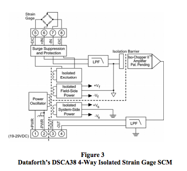
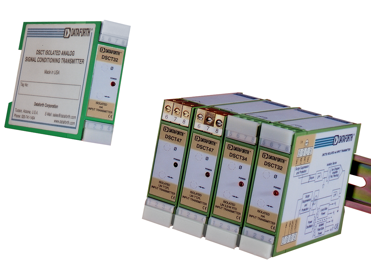
Figure 3 illustrates the 4-way isolation incorporated in Dataforth’s line of high performance DIN isolated analog input signal conditioning modules. These modules accept input analog voltage or current signals from all types of field sensors. Signals are isolated, filtered, linearized, and amplified providing high-level analog levels suitable for data acquisition and control systems. Dataforth’s output modules buffer, filter, isolate, and amplify analog system signals before providing voltages or currents to field devices.

Acknowledgement
Dataforth acknowledges and credits Roger Lockhart, DATAQ Instruments, Inc., for the technical content of this Application Note.

References

1. Dataforth Corp.
   http://www.dataforth.com
2. Application Note AN108
   http://www.dataforth.com/catalog/pdf/an108.pdf