

Signal Conditioning
Dataforth's Signal Conditioning Analog I/O Families
Industrial Signal Conditioning
CONTENTS
- Uses of Industrial Measurement
- Industrial Measurement Environment
- Sensors
- Loops and Analog Signals
- Signal Integrity
- Design Examples
- Product Selection Guide
USES OF INDUSTRIAL MEASUREMENT
There are several distinct uses of analog measurements.
INDICATE-ONLY MEASUREMENTS
Indicate-only measurements are used to indicate the condition of various elements of a process. Estimates place the ratio of indicate-only to control inputs at somewhere between 2-to-1 and 3-to-1. Regardless, these measurements are useful to monitor the condition of intermediary events at every stage of manufacture or processing and may provide necessary information to the plant operator if a control measurement fails. An example of this kind of measurement is the complete temperature monitoring of the distillation trays in a distillation tower. Each measurement is not essential to the control of the side-draw products but does provide valuable insight about the operating conditions and material and energy balances within the tower. They also allow the operator to intervene manually if a control measurement fails.
CONTROL MEASUREMENTS
Control measurements are essential to the economic viability, safety or functioning of a manufacturing process. They provide control over a physical or compositional characteristic of the process. For example, the temperature of a heat exchanger is an essential parameter for both process and safety reasons. Flow measurements and control such as those illustrated by Figure 1: Typical Measurement/Control Loop appear in almost every plant.
CUSTODY TRANSFER MEASUREMENTS
Custody transfer measurements need highly accurate and stable characteristics. These measurements provide information for plant inventory, quantify the amount of material bought or sold between parties or track internal transfers of material from one operating unit to
another within the plant. Frequently the calibration of the instruments is regulated by municipal, state or Federal agencies. The gasoline pump in your neighborhood is an example of these measurements.
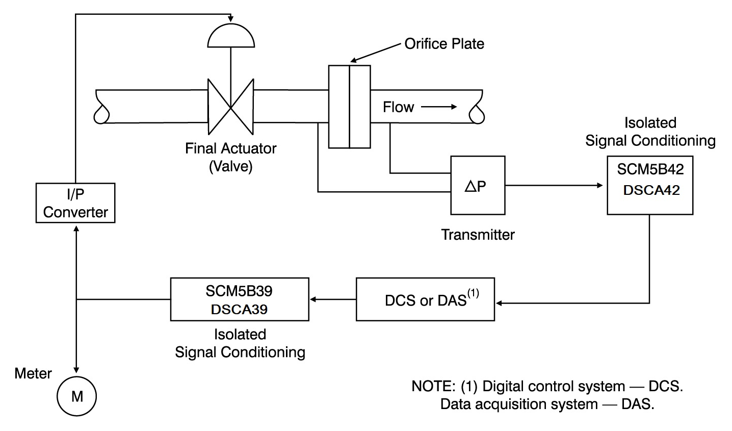
Figure 1. Typical Measurement/Control Loop
ENVIRONMENTAL MEASUREMENTS
Environmental measurements have grown enormously in recent years to provide traceable records of plant effluents, and waste products in compliance with government regulations. An entire technology has evolved to detect and control hazardous materials of all kinds.
SAFETY MEASUREMENTS
Finally, there is an entirely separate and autonomous type of measurement system whose sole function is to monitor and limit dangerous conditions. Measurements include critical process parameters that indicate unsafe operation and potential danger. These systems override the regulatory controls and cause a plant shutdown to a safe status should
emergency conditions dictate. Known as EMERGENCY SHUTDOWN systems, they are frequently equipped with sophisticated events-monitoring recorders so that later analysis of the shutdown events can be made, and future malfunctions avoided or controlled.
INDUSTRIAL MEASUREMENT ENVIRONMENT
Figure 2: Control and Field Conditions — Industrial Measurement Environment shows a simplified view of a measurement and control system. It shows only the essential elements but demonstrates the division between field and control room functions.
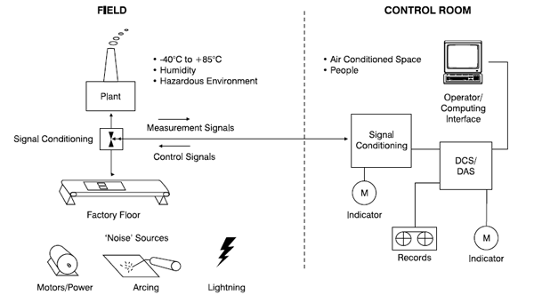
Figure 2: Control and Field Conditions — Industrial Measurement Environment
FIELD
The term ‘field’ refers to the area where the equipment making a product or running a process resides. It is most often the factory floor or the outside areas of an industrial complex such as a chemical plant. What sets it apart from other areas is its harsh electrical and physical environment. The equipment located there is exposed to a much greater range of electrical noise, power surges, temperature, humidity, and corrosive or damaging environments.
The field is where process variables must be measured and where measuring and some signal conditioning equipment must be located. The measuring equipment and wiring may be
near heavy electrical equipment, motor contactors and even lightning. Often the wiring runs several hundreds or thousands of feet, increasing the likelihood of outside interference from this environment.
CONTROL ROOM
The control room is usually a more benign place than the field, with a cleaner atmosphere, air conditioning, and fewer hazardous conditions. However, it also contains electrical equipment and the potential for degrading the quality of measurements. The control room contains signal conditioning and computing equipment that is sensitive to electrical interference.
The control room is usually the location where people interact with the measurement and control systems in a plant. There are exceptions, but the control room is where most decisions about the plant or process are made.
FIELD WIRING
Instrumentation wiring connecting field devices to the control room typically consists of heavy-duty (16-18 AWG) pairs. They are often twisted together to aid in reducing magnetically coupled interference and run with other signal wires in a separate wiring tray away from power distribution wiring. Large numbers of sensor or transmitter signals may be gathered in terminal cabinets located either in the control room area or in an intermediate site for ease of connection to the signal conditioning and display equipment.
In most instances, the cost of wiring is a large percentage of the installed cost of the instru-ment system. This is especially true when the wiring is in or passes through plant areas containing flammable gases or vapors. The hazards represented by these atmospheres force the use of very expensive techniques to prevent fires or explosions caused by an electric spark.
Data concentrators may be used to reduce wiring costs. These devices collect large numbers of signals close to their origins in the field, perform signal conditioning and digital data conversion locally and send the digitized information by communication links to a local area network or to the control room equipment directly.
SENSORS
TERMINOLOGY
The terms ‘sensor’ and ‘transmitter’ are often used interchangeably. However, there is an important difference between sensors and transmitters. A sensor is a device that converts a physical quantity into a form which can be further used to indicate or control the measured variable. This form may be mechanical, like a pressure dial gauge, or may produce an electrical signal. A transmitter takes this idea one step further and provides some manipulation of the sensor signal at the sensor location through amplification, filtering, isolation or other electronic means. For the purposes of this handbook the main difference between sensors and transmitters is that transmitters manipulate the signal at the measurement point. Usually, a data acquisition or control system contains a mix of sensors and transmitters. Ideally, each sensor would have signal conditioning at the point of measurement and transmit a high-level signal back to the data acquisition system or control system. The shorter interconnection from sensor to signal conditioner is less likely to pick up noise, and the high-level output signal offers better immunity against induced pickup from natural or man-made sources. However, this ideal conflicts with the economic reality that signal conditioning at the measurement point is a costlier approach than shared signal conditioning at the data collection/control system. Thus, a compromise must be made between signal integrity and system cost.
SENSOR LINEARIZATION
Many sensors exhibit a deviation from an ideal (linear) relationship between input and output. For example, a given change in temperature does not give rise to the same change in EMF for most thermocouples when measured over different temperature ranges. Sensors or signals which exhibit this behavior are said to be non-linear. A hypothetical non-linear transfer function is shown in Figure 3: Sensor Terminal-Based Linearity. This figure illustrates the concept of ‘terminal-based linearity’ which is the deviation of the actual characteristic from a straight-line coinciding with the actual characteristic endpoint (terminal) values.
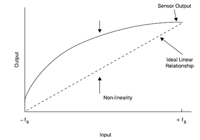
Figure 3: Sensor Terminal-Based Linearity
Most families within the Dataforth product offering – such as the DSCA and DSCT DIN rail products, SCM5B, SCM7B, and 8B SensorLex® plug-in panel products, and DSCT two-wire transmitter products – can be used in the following examples. For simplicity and uniformity, we have referred to the SCM5B family throughout the tutorial.
Several of the Dataforth SCM5B series modules have the ability to create a non-linear transfer function through the module itself. This non-linear transfer function is configured at the factory and is designed to be equal and opposite to the sensor or signal non-linearity. The net result is that the module output signal is linear with respect to a given input parameter such as temperature. An output signal which has been linearized with hardware internal to the SCM5B modules eliminates the need for tedious software routines which determine a linearized signal through the use of high-order polynomials or look-up tables.
A hardware piece-wise linear technique is used in the SCM5B modules to correct the non-linearity of the signal. The difference between the sensor non-linearity and the linearization provided by the SCM5B module is called the ‘conformity error’. This is a description of how well the linearization technique ‘conforms’ to the non-linear curve. Breakpoints are placed along the curve so as to equalize the positive and negative conformity errors. SCM5B modules use 9 breakpoints (10 segments) to correct non-linearity, achieving typical conformity of ±0.015% of span. A normalized plot of sensor non-linearity and hardware linearization is shown in Figure 4: Hardware Piecewise Linearization Using Three Breakpoints. Only three breakpoints are shown in the diagram for simplicity. It should be clear that an increase in the number of breakpoints used will result in a decrease in conformity error.
Linearization of a given input is based upon the input minimum and maximum values. For any input within these limits, the output of the module will be a linear representation of the input. If the input exceeds the minimum or maximum values, the output of the module is no longer a linear representation of the signal. This is also shown in Figure 4: Hardware Piecewise Linearization Using Three Breakpoints. Operation of an SCM5B module beyond the specified input span is not recommended because the output is difficult to calculate and will have increased conformity error. If a standard module input span does not meet customer requirements a custom module can be easily designed for optimum performance in a given system. Dataforth supplies standard models for most thermocouple and RTD types. Consult Dataforth for details on custom modules or non-standard ranges.
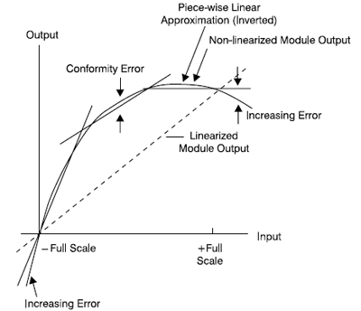
Figure 4: Hardware Piecewise Linearization Using Three Breakpoints
SENSOR CLASSIFICATION
Sensors can be classified in many ways. One method is to separate them into sensors which supply a voltage or current output by themselves and sensors that must have an external voltage or current applied to produce a useful signal. The first type of sensor is called self-excited. The second kind requires ‘external excitation’. These seem like small distinctions, but many sensors require external excitation and the quality of that excitation directly bears on the quality of their output signals. Therefore, the quality of excitation is part of the overall design and application of signal conditioning modules such as the SCM5B, SCM7B, 8B SensorLex®, DSCA series as well as the MAQ20 Data Acquisition System.
Sensors may also be grouped according to the basic measurement they make. Some are straight-forward in their classification, but others can be used for a number of different measurements. For example, the strain gage is really just a variable resistor, but it can be used to measure stress, strain, weight, pressure and acceleration. The most common industrial measurement is temperature.
TEMPERATURE SENSORS
Three types of sensors are most commonly used to measure temperature in industrial environments: thermocouples, resistance temperature detectors (RTDs) and thermistors. Each has its unique advantages, disadvantages and signal conditioning requirements.
Thermocouples (TCs)
Thermocouples are inexpensive, proven sensors and provide the widest range of temperature measurement. TC’s generate their own signal and do not need excitation. They are among the most numerous sensors used.
TC’s do have some drawbacks. Substituting one thermocouple for another one of the same type can produce a slightly different output voltage, forcing recalibration of the signal conditioner for best accuracy.
TC’s may also be contaminated by the environment. This contamination is frequent enough that virtually all thermocouple signal conditioners provide open-circuit or ‘burnout’ detection.
Dataforth’s SCM5B37/SCM5B47,
SCM7B37/SCM7B47,
8B37/8B47,
DSCA37/DSCA47,
DSCT37/DSCT47 thermocouple signal conditioning modules
as well as MAQ20 can be configured for either upscale or downscale burnout detection.
TC operation is based on two physical properties. When a metal rod is heated at one end, a small voltage (Thomson EMF) develops between the hot and cool ends. If two dissimilar metals are joined and heated at their junction but not connected at the unheated ends, a similar EMF occurs. This is called the Peltier EMF. The magnitude and polarity of the Peltier EMF are dependent on the temperatures of the junctions and the combination of the two metals involved.
The algebraic sum of the Thomson EMFs and the Peltier EMF appear at the unjoined ends of the metal pair. This EMF is the basis for all thermocouple operation and is called the Seebeck EMF. If both the joined and open ends of the metallic pair are at the same temperature, this EMF is zero. If the temperatures at the open ends are equal and kept constant, the Seebeck EMF is a direct function of the temperature at the measurement junction and can be used to measure that temperature. The Seebeck EMF depends on the TC’s composition and ranges from 10 to 80mV for full-scale output. See
Table 1: Thermocouple Types for common thermocouples and their measurement ranges.
| TYPE | COMPOSITION | MEASUREMENT LIMITS (°C) |
| J | Fe vs Cu-Ni | -210 to 760 |
| K | Ni-Cr vs Ni-Al | -270 to 1372 |
| T | Cu vs Cu-Ni | -270 to 400 |
| E | Ni-Cr vs Cu-Ni | -270 to 1000 |
| R | Pt-13% Rh vs Pt | 0 to 1768 |
| S | Pt-10% Rh vs Pt | 0 to 1768 |
| B | Pt-30% Rh vs Pt-6%Rh | 0 to 1820 |
| C | W-5% Re vs W-26% Re | 0 to 2320 |
| N | Ni-14.2% Cr-1.4% Si vs Ni-4.4% Si-0.1%Mg | -270 to 1300 |
TC outputs have non-linear relationships (Figure 5: Type 1 Non-Linearity) to the measured temperature. In addition, each thermocouple type has its own non-linear characteristic. This makes it difficult to provide universal linearization for the many types of TCs available. However, Dataforth’s SCM5B47. SCM7B47, 8B47, DSCA47, and DSCT47 series provide hardware linearization and have a complete selection to match all popular TC types.
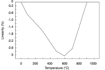
Figure 5: Type 1 Non-Linearity
Thermocouple accuracy depends on the composition and purity of their metals and their fabrication. Usually a thermocouple will not be more accurate than 0.5% to 1% of its total measurement range. This translates to a measurement error as large as 2°C for some TC types. TCs almost always require amplification and cold-junction compensation.
It is important to note that thermocouples always indicate the difference between two temperatures at two junctions. The measurement junction is the one whose temperature is of interest. The other junction is either maintained at a reference temperature (0°C) by physical means or this condition is simulated electronically. It is called the reference junction.
Physically maintaining one or more reference junctions at a constant temperature is not an easy or desirable solution for industrial measurements. Instead, the reference junction is created by bringing the measurement thermocouple wires to the amplifier and connecting them to a terminal block. This terminal block is often called an iso-block (shorthand for isothermal terminal block). Its high thermal conductivity assures that the terminals for the thermocouple wires are at the same temperature. SCM5B modules use the very predictable voltage drop of a silicon diode to measure the terminal block temperature and imitate a thermocouple in an ice bath at 0°C. This entire process is called cold-junction compensation and the circuit is called the cold-junction compensator (CJC).
While the technique sounds complicated, it is easy to implement electronically. Figure 6: Cold Junction Compensation shows a block diagram. The electronic compensation is usually 2-3 times more accurate than the thermocouple itself. It allows precision instrumentation to provide accurate temperature readings even when the ambient (cold-junction) temperature moves through large swings occurring in industrial applications.
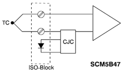
Figure 6: Cold Junction Compensation
Resistance Temperature Detectors (RTDs)
RTD’s are among the most well-behaved and precise temperature measuring devices available for industry. An RTD is a precision resistor with a well-defined resistance vs. temperature curve. RTDs are classified according to their material composition and change in resistance versus temperature (Alpha Value). See Table 2: RTD Types.
| DESIGNATION | MATERIAL | ICE POINT RESISTANCE | ALPHA VALUE |
| PT100 | Platinum | 100Ω | 0.00385 |
| PT200 | Platinum | 200Ω | 0.00385 |
| PT500 | Platinum | 500Ω | 0.00385 |
| PT1000 | Platinum | 1000Ω | 0.00385 |
| D100 | Platinum | 100Ω | 0.003916 |
| SAMA | Platinum | 98.129Ω | 0.003923 |
| NI120 | Nickel | 120Ω | 0.00672 |
| CU10 | Copper | 10Ω | 0.004274 |
Copper, nickel, and platinum RTDs enjoy wide-spread use, although the platinum RTD is now almost universally specified for new industrial installations. The platinum RTD offers many outstanding characteristics including high accuracy, wide measurement range and chemical resistance to many of the nastier atmospheres in industrial applications.
The PT100 is the most commonly used RTD curve and displays an ice-point resistance of 100 ohms. It is based upon several European standards and is supported by the IEC as well. PT200, PT500 and PT1000 RTDs have appeared on the market recently, but they are simply multiples of the basic PT100 curve in their behavior. That is, a PT500 sensor will have five times the resistance of the PT100 at the same temperature. The higher resistance allows use of less material and provides a cost savings. It also can provide a smaller sensor. If, however, the smaller sensor is used, careful attention must be paid to the level of excitation current used. Too much current will cause the sensor’s small mass to self-heat and degrade its accu-racy. Dataforth’s SCM5B34 and SCM5B35 signal conditioning modules specifically use 0.25mA excitation current to eliminate this problem.
The D100 curve is a commonly used US RTD curve and is also supported by a Japanese standard. For many years, the SAMA (Scientific Apparatus Manufacturer’s Association) curve was popular used in the US, but it has since fallen into disuse. The PT100 curve now dominates, finding use in 85-95% of the industrial applications.
RTDs can be used in several configurations that reflect the cost factors and the degree of accuracy desired. Figure 7: Two-Wire RTD Connection (SCM5B34/8B34), Figure 8: Four-Wire RTD Connection (SCM5B35/8B35), and Figure 9: Three-Wire RTD Connection (SCM5B34/8B34) show SCM5B34 and SCM5B35 modules in 2wire, 4-wire, and 3-wire connections respectively. The 2-wire configuration is used when signal lines are short, highest accuracy is not required, and lowest cost of installation is of paramount importance. Because RTD’s must be excited by a current, signal-line resistance will appear in the apparent resistance of the RTD. If the resistance is high, or if the temperature coefficient of the line resistance is high, errors will occur, giving a false temperature reading.
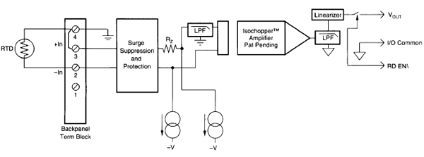
Figure 7: Two-Wire RTD Connection (SCM5B34/8B34)
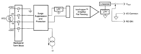
Figure 8: Four-Wire RTD Connection (SCM5B35/8B35)
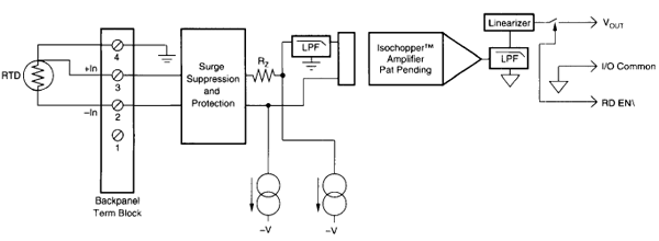
Figure 9: Three-Wire RTD Connection (SCM5B34/8B34)
The most accurate connection method is to excite the RTD by using two power leads to carry the excitation current and using two additional wires to sense the voltage at the RTD directly. If high impedance circuits are used to measure the voltage on the second pair of wires, no appreciable current will flow through them and the voltage measured will only be that at the RTD. This setup, shown in Figure 8: Four-Wire RTD Connection (SCM5B35/8B35), is used in almost all laboratory or other high-accuracy situations. The SCM5B35 and 8B35 are specifically designed for this application.
A reasonable compromise between 2-wire and 4-wire connections is the three-wire con-nection. It offers high accuracy and a lower cost of wiring. This connection is the one most frequently used in factory or plant instrument systems. Figure 9: Three-Wire RTD Connection (SCM5B34/8B34) gives the details. By connecting the wires as shown, equal currents flow from balanced current sources in the SCM5B34 through the ground wire, and back through the top and bottom RTD connections. If the line resistances are equal, the voltage drops from the amplifier inputs to the top and bottom of the RTD will be equal and the error voltages added to each line will also be equal. The two line voltage drops cancel, and the differential input to the amplifier is the actual voltage at the RTD. The voltage drop in the common (ground) wire will be twice that in the other two lines and will add to both amplifier inputs equally. Thus, it appears as a common mode voltage to the amplifier inputs. One may question the basic assumption that the line resistances are equal; using twisted three-wire cable helps make this assumption correct.
One of the few drawbacks to the use of RTD’s is their nonlinear change in resistance with temperature. Figure 10: PT100 Non-linearity shows the nonlinearity of a PT100 RTD measuring from 0°C to 450°C: it is almost 2% of span. Dataforth SCM5B34, SCM5B35, 8B34 and 8B35 modules provide hardware non-linearity correction to 0.015% typical.
The RTD has become the preferred sensor for temperature measurement when accuracy, repeatability and interchangeability are required. The PT100 RTD has a uniform non-linear resistance curve, is resistant to most harsh environments, and is particularly robust for industrial measurements.
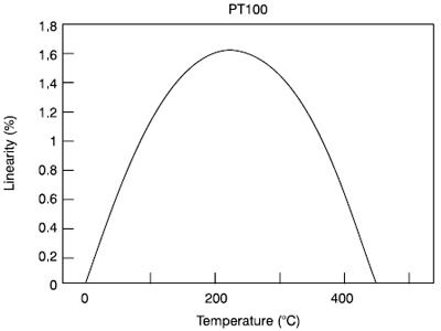
Figure 10. PT100 Non-linearity
Thermistors
Thermistors are relatively inexpensive devices exhibiting very large changes in resistance for small changes in temperature (typically 4-6%/°C). For example, a typical thermistor may have a nominal resistance of 30kΩ at 25°C, but have a resistance of 2.5 kΩ at 85°C. This large change in resistance makes line resistance to the thermistor a very small source of error and use of the thermistor can avoid the three-and four-wire connections common with the RTD.
In the past, thermistors have had very poor interchangeability. That is, an instrument cal-ibrated for one thermistor would require major recalibration when a new thermistor was substituted. Also, the relationship between temperature and resistance could vary significantly from lot to lot and even between sensors from the same manufacturing lot. Low-cost thermistors still retain these characteristics. Today, manufacturers can supply thermistors with vastly improved interchangeability. This fact has given the thermistor a boost as a serious process temperature sensor. This interchangeability has its limitations, however. The temperature span over which interchangeability exists lies between 50°C and 100°C of the thermistor’s total measurement range. As an example, some manufacturers can achieve 0.1°C interchangeability from 0°C to 70°C or from 120°C to 180°C. Thermistors are also somewhat limited in their absolute temperature range. Realistic limits lie between -100°C and 450°C. This can eliminate them from consideration for some industrial measurements, but they still remain ideal for low-cost sensing within their temperature range.

Figure 11. Typical Thermistor Characteristic
Thermistors are very nonlinear devices. Figure 11: Typical Thermistor Characteristic shows the behavior of a typical thermistor. Thermistors can, however, be used in or purchased as part of a resistor network whose output is highly linear over most of the useful temperature measurement range of the device. Figure 12: Linear Thermistor Network shows a resistor-thermistor network whose behavior is quite linear over a modest range as shown in Figure 13: Performance of Figure 12 Thermistor Network. Note that the network resistance now approaches that of some RTDs, and the three- and four-wire connections used with RTDs may be necessary for best accuracy. Dataforth offers several signal conditioning modules for thermistors. Because of the large variety of thermistors available, consult Dataforth for details.
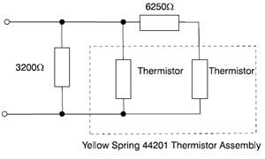
Figure 12. Linear Thermistor Network
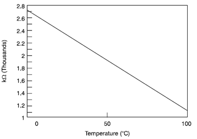
Figure 13. Performance of Figure 12 Thermistor Network
One of the big advantages of thermistors is their small size. This gives them perhaps the best thermal response time of almost any temperature sensor. Some can react in milliseconds to large temperature variations. The downside of this small mass is self-heating of the sensor from the excitation current. This heating can pose a significant source of error. Since thermistors are typically high-resistance devices, large currents will produce large self-heating errors. Pay close attention to the manufacturer’s recommendations in this area.
MOTION SENSORS
Motion sensors are useful in a number of different applications. The two most common motion sensors are based on changes in resistance. These are the slidewire and strain gage. Another fairly common motion sensor is the accelerometer, which is used to measure dynamically changing motion. All of these sensors are very broad in their applications. For brevity, they will be treated from an interface and signal conditioning viewpoint only. Specific measurements and techniques will not be discussed.
Slidewire
A rotary or linear resistor may be used to sense motion. This motion can be the small displacement of a pressure diaphragm, the stroke of an hydraulic piston or shaft rotation. If voltage excitation (5 - 10VDC) and a potentiometer connection are used, the output will be a fraction of the excitation voltage and the measurement is referred to as a slidewire measurement. These signals usually are 0-5VDC or 0-10VDC. If the motion being measured is non-linear, the relationship between motion and resistance of the sensor can be manufactured to provide a linear signal. If constant-current excitation and a rheostat are used, the resistance change can be scaled into almost any engineering unit. For example, linear resistors are available in 1 to 20-inch lengths. The resistance of these devices is usually a constant value per inch. As an example, if that value is 1kΩ/inch, and a 0.25mA current is used, linear measurements could be made for distances between 1 and 20 inches. The scale factor would be a constant 0.25VDC/inch regardless of the physical length of the linear resistor. See Figure 14: Slidewire Example.
Slidewire sensors provide an inexpensive solution for many measurement problems. Their main faults are noise introduced by the sliding contact and wear of the resistance element. If the measured variable changes by small amounts, the sliding contact is fairly stationary. The small changes that do occur cause a scrubbing action at a single point on the element. A clear example of this problem appears in the data sheet of any slidewirebased pressure sensor where the sensor will be lifetime rated in numbers of pressure cycles. Since most slidewire sensors measure slowly varying variables, the low bandwidth of the SCM5B36, SCM7B36, 8B36, DSCA36, and DSCT36 potentiometer input modules are particularly useful in eliminating contact noise. These modules also supply constant-current excitation suitable for these sensors. Mechanical wear can be addressed only by replacement of the sensor.
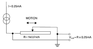
Figure 14. Slidewire Example
STRAIN GAGES
The strain gage is a special adaptation of the resistive motion sensor. Rather than moving a contact along the resistor, the strain gage itself is lengthened or shortened. The resistance of a conductor is proportional to its resistivity and length and inversely proportional to its cross-sectional area. As the wire is stretched, its length increases, and its cross-section gets smaller. Both of these changes increase its resistance.
If the wire had been placed in tension and then relaxed, its resistance would decrease. The change in resistance for small changes in length is directly related to the tension in the wire. This effect is not precisely linear but is very repeatable. Gages made with stretched conductors have measured the elongation or contraction of bridge structures, the flexure of aircraft wings, and the stress and strain in the airframe of the Space Shuttle. They have also been used for more than a half century to make pressure, force, weight, and acceleration measurements.
Practical Gage Arrangements
The strain gage converts all of these physical quantities into a changing resistance by responding to the stress or strain induced in a mechanical member to which it is attached. For example, a pressure diaphragm stretches inward when pressure is applied. This motion stretches or contracts a strain gage attached to the diaphragm and increases or decreases its resistance. Measuring the resistance provides a corresponding measure of the pressure.
The change in resistance of a strain gage is small and a method of detecting the change is more useful than measuring the total gage resistance. Figure 15: Quarter Bridge Strain Gage shows the most common way to detect the change. The strain gage is connected as one arm of a Wheatstone bridge. An excitation voltage or current is applied and the bridge is initially balanced for zero output. As the gage is stressed or strained, the bridge unbalances by the change in gage resistance. This can be detected by a sensitive voltmeter connected across the center arms of the bridge. Further sensitivity (more output) results when two or more of the bridge resistors are ‘active’. Also, using two- or four-arm active bridges result in a more linear signal. Figure 16: Strain Gage Connections to Signal Conditioning Modules (SCM5B38) shows quarter, half and full bridge arrangements when connected to SCM5B38 strain gage modules. Opposing arms are placed in tension and compression (stressed and strained). The full bridge will produce four times the signal of the quarter bridge and its output will be electrically linear with the change in resistance of the identical arms. The success of the sensor designer in producing identical stress/strain in each of the bridge arms determines how linear the signal will be with changes in the physical quantity. Practically, strain gage manufacturers are able to achieve this goal within 0.1-1.0% accuracy.
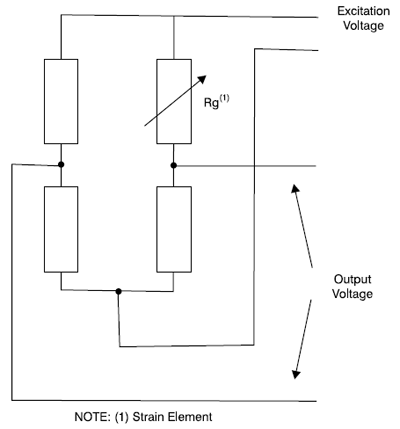
Figure 15. Quarter Bridge Strain Gage
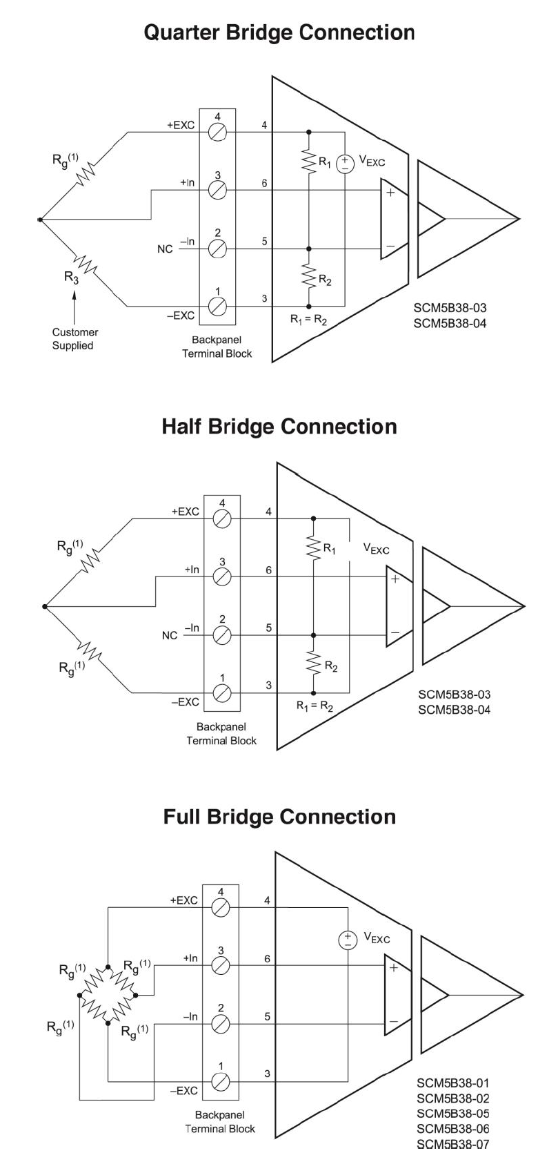 Figure 16. Strain Gage Connections to Signal Conditioning Modules (SCM5B38)
Gage Types
The original wire-based sensor has not been used industrially for a long time. It has been replaced by a number of strain elements that work in the same way but offer advantages of cost, accuracy, lower power consumption or a combination of these factors.
Bonded strain gages are metal film resistors mounted on carriers or substrates. These sub-strates attach to the stress member with adhesives. Because the adhesive does not perfectly affix the strain gage to the stress member, bonded gages are subject to a phenomenon called ‘creep’. Minute shifts of the gage(s) on the stress member appear as small drifts in zero and full scale calibration. Bonded gauges require relatively large amounts of power (5-10VDC, 25-125mA). These are not insurmountable problems, and the manufacturing and signal processing technology available for these types assure a quality measurement. Nonetheless, these and other traits have led to greater use of piezo-resistive silicon and vapor-deposited metal film strain gages.
The silicon gage combines the stress member and strain element in one single structure. The silicon gage has no intermediate materials and pure silicon makes a very good stress member: It has nearly perfect elasticity and has about 10 times the output of a bonded gage while using less power. It also is an inexpensive gage to manufacture.
The disadvantages of silicon strain gages arise from material limitations and temperature sensitivities of the resistors. Silicon functions well as a gage material between -100°C and 200°C. Silicon cannot withstand exposure to many chemicals or corrosive atmospheres and must be protected by other materials. This raises the cost of some sensors based on the silicon gage. Silicon gages display strong zero and full-scale temperature dependencies. Sensor compensation techniques can largely make up for these dependencies but add a small cost penalty.
Vapor-deposited strain gages offer a compromise between the monolithic structure of the silicon gage and the advantages offered by the bonded film gage. This gage is formed directly on the surface of the stress member by first vapor-depositing a substrate on the stress member and then vapor-depositing a metal film pattern onto the substrate. This method provides a structure that is nearly as monolithic as the silicon gage. Also, the materials used withstand higher temperatures. By controlling the amount of metal film deposited, the resistance of these gages can be adjusted to between 3-15kΩ for low power consumption. This makes the vapor-deposited gage strong competition for the silicon gage, especially in 4-20mA transmitters.
The disadvantage of this technology lies primarily in its low output voltage — a trait it shares with the bonded strain gage. However, because it can be fabricated in batches and laser-trimmed for final zero and full-scale sensitivity, this gage offers many of the low-cost advantages of the silicon gage and exhibits smaller temperature effects than the silicon gage.
The signal conditioning used with strain gages must provide exceptionally stable excitation and high sensitivity. Some bridges provide as little as 6.667mV full scale output when excited with 3.333VDC (20mV at 10VDC excitation). The stability of the excitation source directly controls the stability of both zero and full-scale output. The Dataforth SCM5B38 offers the excitation stability required and provides stable gain for processing of these low-level signals. An additional bonus is the isolation of the excitation source from the rest of the module. It is immune to line-voltage and transient damage. It is also less sensitive to bridge loads than most available modules.
Accelerometers
Accelerometers fall into two general classes. The first is based on the strain gage in one of its many forms. In this sensor a mass is attached to the stress member and exerts a force proportional to the acceleration which it experiences. A strain gage then converts this stress into an electric signal. The output of the strain gage is handled just as it is for a pressure or force measurement. Accelerometers made in this fashion are able to measure extremely low rates of change in acceleration but tend to be limited in bandwidth. This limit may be as high as 25kHz.
The second type of accelerometer makes use of the strong piezo-electric effect displayed by some crystalline and ceramic materials. Under deformation, these materials develop a voltage. This effect can be used to measure the force experienced when a mass attached to these materials accelerates. Because these materials are good insulators, they behave electrically like a capacitor in series with a voltage and little or no current can be drawn from them without losing accuracy. The capacitance of a long cable can severely affect their measurement characteristics. Therefore, piezo-electric sensors are usually amplified directly at the sensor. Since the voltages available from these devices can be very large, the amplifier is usually an impedance-matching device. That is, it provides a very high impedance (resistance and capacitance) to the sensor and provides a low-impedance output able to drive long cables. See Figure 17: Charge Amplifier for an accelerometer which could be used for bearing vibration (seismic) monitoring.
Figure 17. Charge Amplifier
High frequency response (100kHz-300kHz) can be achieved with piezo-electric accelerometers, but they tend to be very limited at low frequencies. Constant improvements are being made, so be sure to check manufacturers’ specifications.
LOOPS AND ANALOG SIGNALS
Sensors are connected to signal conditioning equipment, data acquisition or control systems, and control devices. This collection of equipment is known in the industry as a measurement loop or, simply, a loop. An example of a such a loop was shown in Figure 1: Typical Measurement/Control Loop. A loop may be classified by the measurement it is making, by its use, or by the type of elec-tronic signal carrying the measurement between the sensor and the rest of the equipment. Except for purely digital systems such as FIELDBUS, loops make use of voltage, current or frequency signals. Most use voltage or current. The amount of power required to make the measurement or to power the sensor influences the choice of loop configuration. For example, a gas chromatograph used for chemical analysis requires more power than is available from a 4-20mA loop and is usually mains-powered in a four-wire configuration. Other measurements are self-excited or can be powered by low energy sources. In this case, two-wire transmission offers cost advantages regarding wiring costs and simplifies the use of intrinsic-safety techniques, saving further in installed cost.
MEASUREMENT LOOP CONFIGURATIONS
Measurement loops are configured in one of three ways: two-wire, three-wire and four-wire. Some loops do not require excitation or local signal conditioning or have outputs which may be handled directly by the data acquisition system. Examples of the former are thermocou-ples, while the latter are represented by potentiometers driven by pressure elements. The greater number of measurement loops do require some form of local excitation and signal conditioning. Merits of each signal conditioning configuration vary according to the needs and cost-sensitivity of the application.
Four-Wire Loops
Four-wire loops (Figure 18: Four-Wire Loop) provide the greatest degree of flexibility because they are supplied with power independent of the signal return lines and are therefore not limited in power consumption or by signal ground induced errors. These reasons are the primary ones for choosing this configuration. They do impose a cost penalty because they cannot be easily installed using intrinsically safe techniques and do require the running of extra wiring, which is a major cost in instrument loop installation. However, for some meas-urement devices, the four-wire loop is the only alternative. Some sensors and all analyzers simply require too much power to be run in less costly configurations.
Figure 18. Four-Wire Loop
Three-Wire Loops
Three-wire loops (Figure 19: Three-Wire Loop) offer some of the flexibility of the four-wire configuration and the savings and simplicity of one less wire to install. They do suffer from a certain inflexibility in that both power and signal ground are shared by the same wire. If sub-stantial power or long line lengths are involved, the voltage drop (I x RRETURN) in the shared ground return can substantially interfere with the accuracy of voltage-mode signal transmission. In current-mode and frequency-mode signal transmission, this constraint can be avoided.
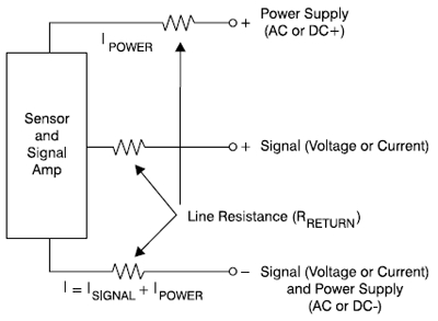
Figure 19. Three-Wire Loop
Two-Wire Loops
When considering two-wire loops, most people think of the 4-20mA loop, but other measurements fall into this category also. These other cases involve any sensor which generates its own signal and could include the thermocouple, pH, and ORP (oxygen reduction potential) sensors. These sensors operate in the voltage mode, usually have output signals of moderately low-level (0-500mV), and are very susceptible to induced noise. These sensors experience impedance restraints regarding either leakage resistance in the instrument wiring or input characteristics of the signal-conditioning input.
The current-mode, two-wire configuration (Figure 20: Two-Wire Loop) overcomes many of these constraints. It allows local signal conditioning, and because it operates in a manner that is relatively immune to induced noise, has become the de facto standard for most critical process-control measurements. This configuration also enjoys economic advantages arising from reduced wiring costs and the ability to easily use intrinsically safe installation practices.
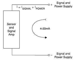
Figure 20. Two-Wire Loop
It does impose constraints on the designer of both the transmitter and data collection equipment. First, the transmitter must perform all functions within a limited power budget.
Sensor excitation, amplification and signal conditioning functions must be accomplished with 4mA or less at voltages typically ranging from about 12 to 36 volts. At the receiver, the signal usually must be converted into a voltage and level-shifted to a zero-based range so that subsequent conversion into digitized format may be done using the full input capability of the analog-to-digital converter. Both the current-to-voltage conversion and level-shifting can intro-duce extra errors in both zero and span if proper care is not given to circuit design.
ANALOG SIGNALS
Voltage-Mode Loops
Voltage-mode loops present to the data acquisition system a voltage proportional to some physical measurement. The nature of the voltage source, its impedance, length of wiring, and the nature of the receiving instrumentation all affect the accuracy of the final measurement. Figure 21: Typical Voltage Loop shows some of the elements to consider when using a voltage-mode loop. The representation is general and does not reflect whether the voltage loop is 2-, 3- or 4-wire in nature.
The measurement voltage may be directly from a self-exciting source (e.g., thermocouple) or from a signal conditioning amplifier. Each voltage source will have some internal impedance which acts as if it is in series with the actual signal. The signal lines will also have some small impedance, and the receiver will present some load to the voltage signal. These elements are shown as lumped components in Figure 21: Typical Voltage Loop. The sensor, line and receiver impedances form a voltage divider that can affect the overall accuracy of the measurement. For this reason, the receiver impedance is made as high as possible. For thermocouple, RTD, or strain gage measurements (about 10-300mV) or for preconditioned signals, the required impedance is of the order of 100MΩ. For pH, ORP, accelerometer or photo diode applications, the receiver impedance must be greater than 200MΩ. In these latter applications, the effects of humidity and integrity of wiring on cable leakage resistance make signal conditioning at the point of measurement almost imperative.
Because voltage-mode loops operate at relatively high impedances, their chief susceptibility to noise arises from electric fields and ground potential differences. Electric fields arise from nearby natural or man-made sources. The most common sources include power equipment and switching power supplies. Use of receiver designs offering high common-mode rejection and common- and normal-mode filtering offers a measure of immunity, while appropriate shielding of signal lines decouples the signal lines from the interfering source. Using point-of-measurement signal conditioning to raise the level of signal voltage improves the ratio of measurement signal to interfering noise.
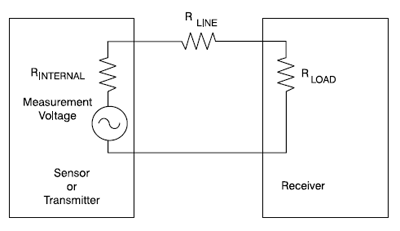
Figure 21. Typical Voltage Loop
Ground potential differences create potentially larger interference than electric fields because they cannot be easily shielded against and because many sensors are tied to local ground. Typical sensors for which this is true are thermocouples and pH or ORP probes. This local ground can, on a transient basis, be several hundred volts different from the ground potential at the receiver. A plant grounding system designed at the time of plant construction can be of benefit but is often not available in old or retrofit installations. Use of receivers with high common-and normal-mode rejection also offer some help in these difficult situations, but transformer isolation provides the greatest relief from this problem. When in doubt, isolate!
Among the chief advantages of voltage-mode loops is their ability to be multiplexed directly. The expensive signal-conditioning and data conversion equipment can be shared with many loops, reducing the per-loop cost of these functions. In most configurations, they do not require zero offsetting and don’t need a precision resistor for conversion of current to voltage.
Current-Mode Loops
Current-mode loops offer relatively high immunity to electrostatic interference but are susceptible to magnetically-induced errors. The simplest way to avoid these errors is to use twisted pair signal lines and to maintain separation from power or relay control lines or other sources of magnetic induction. As with voltage-mode loops, current-mode loops can also suffer from ground potential problems. Again, transformer isolation is the best remedy.
While current-mode loops offer the better noise immunity of the two types, they do require additional conversion into a voltage at the receiver, and most often require level-shifting to return them to a zero-based voltage signal. In particular, the two-wire 420mA loop is difficult to multiplex directly because of the need to keep power on the loop to avoid amplifier settling-time problems. Figure 22: Typical Current Loop shows a typical current loop configuration. Also, most multiplexers experience difficulty with the power supply voltages used in these loops. The conversion and level-shifting is often performed before multiplexing occurs. This imposes an additional cost at the receiver. Even so, for many critical control applications this loop type has become standard because of its superior noise immunity.
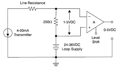
Figure 22. Typical Current Loop
Frequency-Mode Loops
Frequency signals are used less often than voltage or current signals but do offer some distinct advantages. A frequency signal is essentially a digital signal and is relatively insensitive to noise and interference from outside sources. It is sometimes used for this reason alone. However, there are some sensors that inherently generate a repetitive pulse train. Such sensors as turbine meters, flowmeters based on vortex shedding, or totalizers are ‘natural’ for frequency transmission. Dataforth’s SCM5B45, 8B45, DSCA45, and MAQ20-FREQ Frequency Input modules can accept either TTL level or AC signals and convert their frequency into a proportional 0-5VDC or 0-10VDC output. Full scale inputs as high as 100kHz are supported.
Choice of Signal Level
While there is no universal rule for choosing the type and level of signal input to the receiving equipment, there are some practical considerations where large numbers of measurements must be dealt with. First, the wiring costs, including labor, are a major part of the cost of ownership of instrumentation. Second, the ability of the system to detect abnormal wiring situ-ations such as opens, or shorts is often crucial. Third, with lost-production costs in modern plants running from $20,000 to $500,000 per hour, it is prudent to repair by replacement and then fix the defective piece of instrumentation off-line. This is possible only if spares are at hand. Standardization on one or two input types reduces the costs associated with carrying the spares inventory of instruments and input modules. Table 3: Common Signal Types and Levels lists many of the standardized signal levels in use today.
| SIGNAL TYPE | STANDARD RANGES |
| Voltage | 0 through 500mV (non-standard ranges for TC’s, RTD’s and others) 0-1V 0-5V 1-5V 0-10V ±1V ±2.5V ±5V ±10V |
| Current | 0-1mA 0.2-0.5mA 0-20mA 4-20mA 10-50mA (obsolete, but still in use) |
| Frequency | 0-500Hz throught 0-100kHz Full Scale (no standards adopted) |
SIGNAL INTEGRITY
There are many pieces of equipment in both the field and control room that can interfere with measurement signals. This equipment and other sources of man-made and natural ‘noise’ are a part of the ‘electronically hazardous’ environment in which instrumentation exists. Since the equipment and natural events themselves cannot be eliminated, their effects upon the instruments must be understood and minimized or eliminated. By understanding the ways in which this noise gets into the instrument system, one can take rational steps to avoid problems in a new system or eliminate them in an existing one. Table 4: Sources of Error and Possible Solutions list the most common problems and possible solutions.
| ERROR SOURCE | POSSIBLE SOLUTIONS |
| Capacitive Coupling | Shielding Cable spacing Twisted Pair |
| Magnetic Coupling | Twisted Pair Cable Spacing Eliminate ground loops Shield Grounding Isolation |
| Ground Loops | Correct Shield Grounding Isolation |
| Over-Voltage and Transients | Shielding Isolation Care in Installation — Avoid Improper Connections Equipment Selection Cable Spacing |
| EMI/RFI | Shielding Twisted pair Equipment Selection |
| Aliasing | Front-end Filters Equipment selection System Design — Chose Correct Sampling Rate |
SOURCES OF ERROR
Each of the following influences can seriously degrade signals. Methods to avoid or minimize their effects are discussed in later sections.
Capacitive Coupling
Any piece of plant equipment can develop an electric charge. So long as this charge does not change, it has little or no effect on an instrument system. However, all electrically powered equipment has a varying charge or voltage. It can vary in a smooth or erratic (transient) manner. When it does so, the equipment creates a changing electric field that can capacitively couple into the sensor, its signal conditioning equipment or its wiring. Man-made static discharges and lighting have been known severely damage instruments.
Magnetic Coupling
An electric current produces a magnetic field. If a conductor moves through the magnetized field, a current is produced in the conductor. Similarly, if the electric current in a conductor varies, a current is induced in nearby stationary conductors. The resulting induced current can be a disturbing influence or can produce a voltage across the ends of the conductor, also producing an influence. Since most sensor wiring is fixed in place, varying currents are the usual cause of magnetic coupling in instrumentation systems. Often these current influences result from placing wires too close to power conductors.
Ground Loops
Ground is an elusive and often misunderstood electrical concept. Its very name implies that the soil we walk on is the place to which all currents and voltages are somehow referred. In an electric power distribution system, a rod driven into the earth or a buried metal pipe is ‘ground.’
Unfortunately, that is not the entire the story. The local ‘ground’ where you are now located can be several volts above or below that at the nearest building or structure. If there is a nearby lightning strike, that difference can rise to several hundreds or thousands of volts (Figure 23: Differences in Ground Potential). Even in a home, different parts of the electrical grounding system can vary by several volts. This arises not only from the resistance of wiring but its inductance. If the currents change very rapidly, the voltage drops in the ground system will approach several hundred volts for short periods of time. For example, studies conducted by power companies have shown that the operation of an oil burner ignitor can produce tran-sient differences up to 2000 volts routinely. Imagine the potential for similar voltage spikes in other industrial environments.
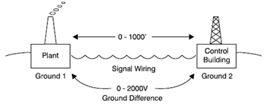
Figure 23. Differences in Ground Potential
The voltages themselves can obviously provide a great source of interference for a measurement loop, but the currents which cause them can also induce significant currents and voltages in the signal wires located nearby. Circulating currents in ground loops may also be periodic in addition to being transient events. Consider the case when a ground loop is formed with AC power lines such that a 50 or 60Hz signal is imposed on the gound loop. If the measurement signal ground is part of the ground loop, the unwanted AC signal will appear as an error voltage or perhaps as a common mode signal to the system inputs. Figure 24: Ground Loop Signal Protection shows a 10mV thermocouple signal which is corrupted by a 60Hz and a 180Hz (3rd harmonic) ground loop voltage. The original signal has been corrupted beyond recognition. Proper grounding practice and use of a signal conditioner with high common mode rejection is vital in preserving signal integrity (Figure 25: Ground Differences Cause Uncertain Results).
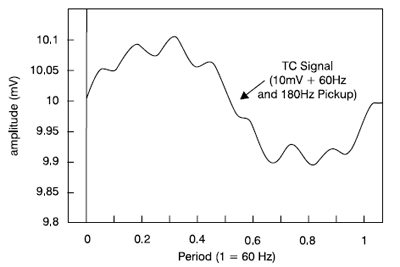
Figure 24. Ground Loop Signal Protection
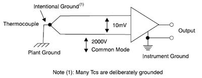
Figure 25. Ground Differences Cause Uncertain Results
Over Voltage and Transients
Beside the transient voltages caused by ground potential differences, large voltages can appear in the signal wiring directly. This can arise from capacitively or magnetically induced sources, from accidental electrostatic discharges or from nearby high-voltage arcs such as welding. Some of the instrumentation installed in today’s industrial plant is wired in close proximity to power wiring. Although this is very poor instrument wiring practice, it does happen. Accidental connection of signal conditioner inputs to 110 or 240 VAC is not an uncommon event.
Many manufacturers of industrial equipment provide input circuit protection to prevent damage from transient voltages and the misapplication of power line voltages. Such abnormal voltages will render the measurement useless during the time they exist but will not damage the equipment if it has this protection. When specifying signal conditioning equipment, choose equipment that provides SWC (surge withstand capability) protection and line voltage protection. Compliance with EN61000-4-2 ESD Immunity and ANSI/IEEE C37.90.1 standards are a good indicator that the equipment supplier has provided adequate protection (Figure 26: EN61000-4-2 and ANSI/IEEE C37.90.1-1989 Test Waveforms). All Dataforth signal conditioning products are designed to meet this specification.
Following Table 5: Waveform Parameters lists the waveform parameters for Figure 26: EN61000-4-2 and ANSI/IEEE C37.90.1-1989 Test Waveforms
| Level | Indicated Voltage [kV] | First peak current of discharge ±10 % [A] | Rise time tr with discharge switch [ns] | Current (±30 %) at 30 ns [A] | Current (±30 %) at 60 ns [A] |
|---|---|---|---|---|---|
| 1 | 2 | 7.5 | 0.7 to 1 | 4 | 2 |
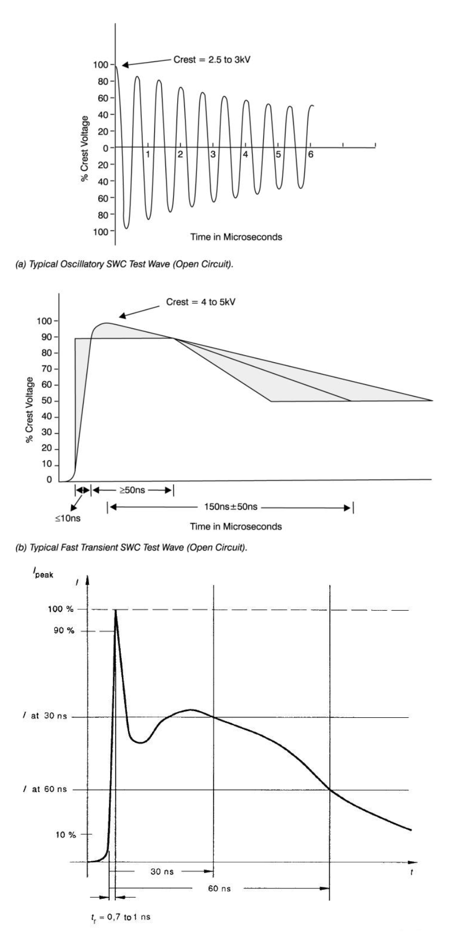
Figure 26: EN61000-4-2 and ANSI/IEEE C37.90.1-1989 Test Waveforms
EMI and RFI
Electromagnetic interference (EMI) is a general term for induced errors signal loops are subjected to. It includes most of the sources discussed before. However, it has come to have a somewhat more restricted usage in the instrument business. It has become synonymous with the term RFI (radio frequency interference). The usual source of this particularly annoying disturbance is a radio transmitter. If it is from a nearby radio or television station, it can at least be diagnosed with some ease. More often it appears as a ‘random’ or intermittent change in the measurement signal. In this situation, the usual sources are transmitters or two-way radios used in the plant. The normal signal conditioner will not amplify these signals because they are too high in frequency. However, the input stages of some signal conditioners will rectify the RF voltage in a similar to the old ‘crystal’ receivers. The rectified voltage appears as a drift or sudden shift in the measurement signal (Figure 27: Electromagnetic Interference). Two-way radio conversations between the field and control room locations can cause seemingly random changes in signal levels. Look for signal conditioning equipment that specifies EMI/RFI immunity. Per EN61000-6-4, a typical specification might state “less than 0.5% shift in the presence of 10V/m electromagnetic fields.
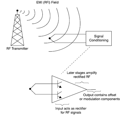
Figure 27. Electromagnetic Interference
Aliasing
‘Aliasing’ becomes an issue when signal conditioning passes from the purely analog world to the digital world. This, of course, is the norm in today’s systems. The notion of aliasing is confusing to some users of data acquisition equipment. The need to prevent aliasing arises from the use of analog-to-digital conversion in the signal conditioning path.
To understand the problem, consider the data conversion system shown in Figure 28: Aliasing Errors. This is not a real system, because one does not usually re-convert a digital signal as shown. However, reconstructing an analog signal after it has been converted allows us to see the aliasing phenomenon directly in the frequency domain. The input signal contains two frequency spectra centered around f1 and f2, as shown in Figure 28: Aliasing Errors. The sampling frequency is fs. The output spectrum for this system is shown in Figure 28: Aliasing Errors. The term ‘Nyquist frequency’ comes up often in discussions about data conversion systems. It’s simply the sampling frequency divided by two and represents the highest signal frequency which can be processed in a perfect system without aliasing.
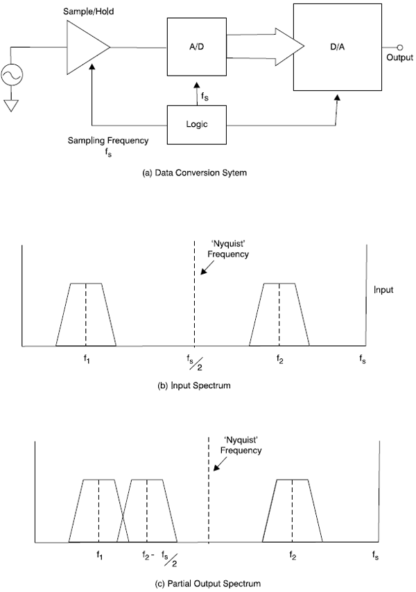
Figure 28. Aliasing Errors
Signals, such as f2, that are above the Nyquist frequency are present in the output sprectrum, but also appear in the output at a lower frequency. These output signals are false rep-resentations or ‘aliases’ of the higher frequency input signals. Obviously, this is not a faithful reproduction of the input signal and can lead to large signal distortions if not handled properly.
WAYS TO PRESERVE SIGNAL INTEGRITY
Signal integrity begins with a quality measurement and good signal conditioning equipment. Despite the best equipment, however, signals can be degraded if the equipment is not properly installed. Signal integrity is profoundly affected by shielding and wiring practices. It can also be affected by system design choices.
Shielding
Cable shielding is used to minimize or eliminate capacitively coupled interference and to aid in lowering RFI-induced errors. Shielding is arguably the most controversial subject faced by instrument users. Some say ground everywhere; others say ground only at the source end and others defend grounding at the receiving end. The most constantly ‘correct’ place to ground an instrument wiring shield is at the receiver end. However, some manufacturers of transmitters and receivers supply cables with shields connected at the source and, short of remaking the instrument, there is no choice but to accept this ground for the shield. One important rule is that there should be only one ground for the shield. Violating this rule automatically creates a ground loop and all of the problems associated with it.
Shielding consists of a metallic sheath surrounding the instrument wires. This is intended to be a Gaussian or equi-potential surface on which electric fields may terminate and return to ‘ground’ while leaving the internal wires uncoupled to these fields. But, if two grounds exist, ground currents will flow through the shield which generate mag-netically-induced voltages in the signal leads. The shield meant to reduce capacitively coupled errors has become a source of magnetic fields and introduced an additional source of error. Avoiding this is as simple as following the rule above: use only one ground in the system (Figure 29: Single Point Ground).
Sometimes the installation and mechanics of the wiring do not allow the one-ground approach. In that case, two steps help: use twisted signal wire pairs and isolation.
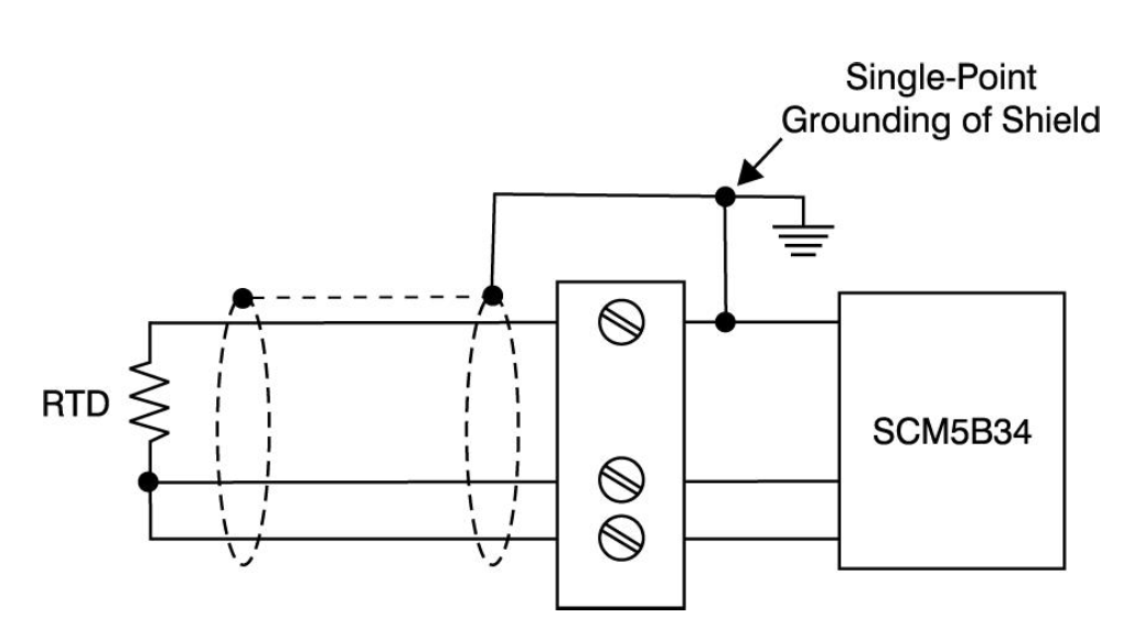
Figure 29: Single Point Ground
Twisted Pairs
Using twisted wire pairs is the simplest way to reduce magnetically induced interference. This applies for shielded or unshielded wires and and for cases where the field is caused by shield currents or from other field sources. The induced voltage is proportional to the magnetic field strength and to the wire loop area through which it passes (see Figure 30: Twisted Wire Pairs Reduce Magnetically Induced Errors). Twisting the wires forces them close together, reduces the loop area and lowers the induced voltage.
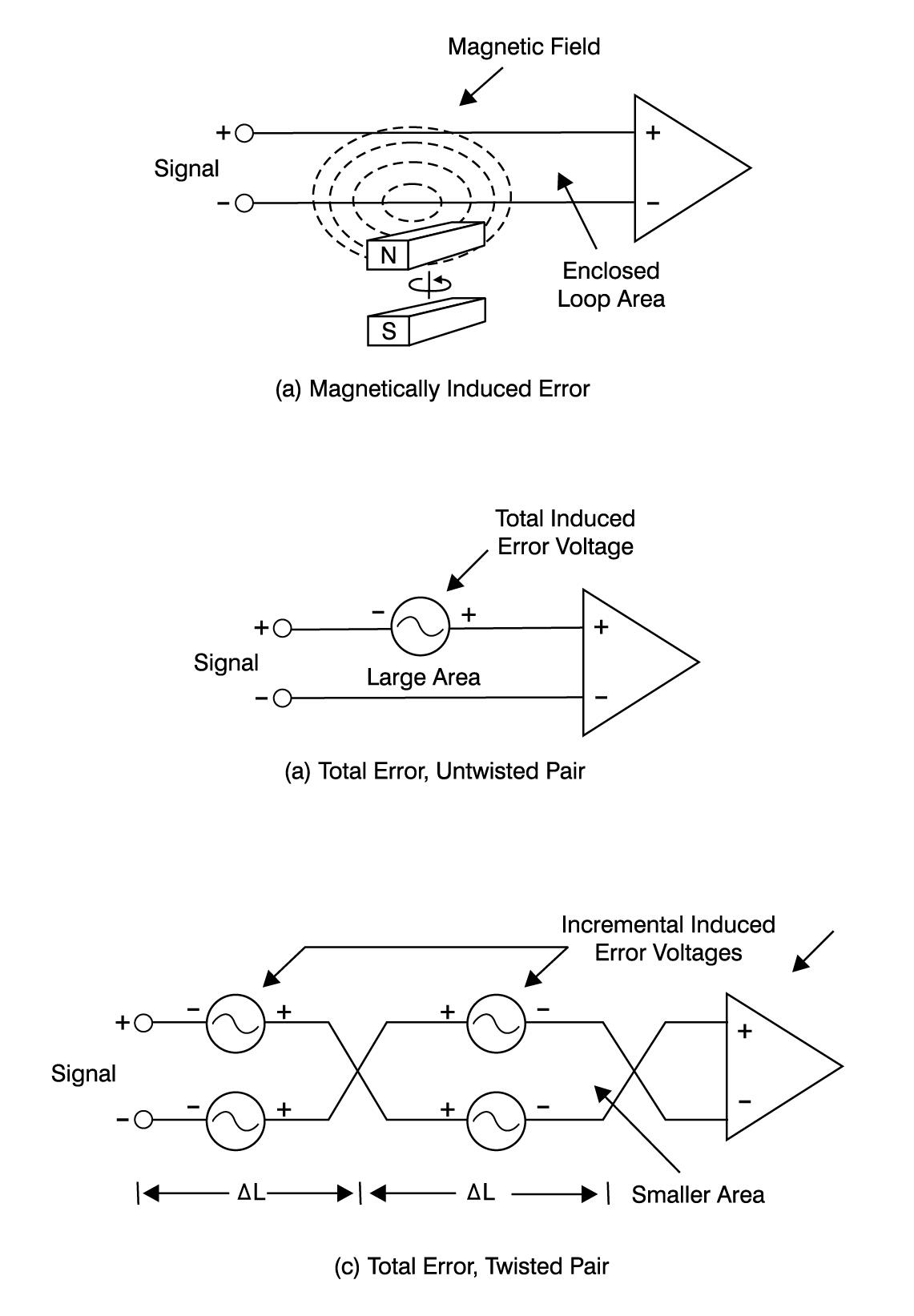
Figure 30: Twisted Wire Pairs Reduce Magnetically Induced Errors
Another benefit of using twisted pair is more subtle. By alternating the positions of the wires in an electric field, the induced voltages in each incremental length of wire tends to cancel the voltage in the adjoining lengths of wire. Figure 30: Twisted Wire Pairs Reduce Magnetically Induced Errors shows an untwisted pair with all induced voltages portrayed as one voltage source, while Figure 30: Twisted Wire Pairs Reduce Magnetically Induced Errors shows the total effect of twisting the wires. The enclosed magnetic loop area has been reduced dramatically and magnetically induced errors are much reduced. Pickup from an electric field has also been reduced. Each incremental length of wire has its own voltage error from this source, but these errors oppose each other and tend to cancel.
Cable Spacing
When cables are located in close proximity, coupling can cause unintended pickup from the voltages and currents running nearby. It is often tempting to use the same conduit or cable tray to run instrument wiring with power wiring. Don’t do it! This practice is a sure formula for added difficulty with instrumentation signals. Keep the instrument wires together and apart from all power wiring.
Isolation
Isolation is a universal way to eliminate ground loop problems. Isolation simply means using one of a number of electronic techniques to interrupt the connections between two grounds while passing the desired signal with little or no loss of accuracy. Without a path for ground currents to flow, these currents cannot induce signal errors. Isolation also solves the other problem encountered with ground loops — voltage differences which cannot be rejected by the signal conditioner. Isolation has become very cost effective for solving many signal conditioning problems and is an integral part of each SCM5B module.
Anti-Aliasing Filters
Earlier, the phenomenon known as aliasing was examined. The aliased signals resulted from higher-frequency signals in the input. A front-end low pass filter would prevent higher frequencies from being processed and prevent aliases from appearing in the output spectrum. The sharper the cutoff of the low-pass filter, the smaller the amount of aliasing. Practically, there will always be some aliasing. It just needs to be reduced to insignificant levels. The six-pole low-pass filters used in the SCM5B series exhibit superior performance in rejecting higher-frequency signals and minimizing aliasing.
The sampling frequency of a data conversion system also has a profound effect on aliasing. It should be significantly higher than that of the desired input signals — usually 3-10 times the spectrum of the desired signals. How much higher is strongly influenced by the characteristics of any input filtering.
Note that digital filtering in the data acquisition system will not reduce or eliminate the aliasing. The aliased signal is converted into the spectrum of the desired signal and the digital filter cannot distinguish between the real and aliased signals. Once aliasing occurs, the original input signal has been lost and cannot be recovered by any means.
DESIGN EXAMPLES
The following design examples illustrate one or more common signal conditioning or installation problems and show how improvements can be made. The examples shown are real installations. The remedies were achieved using readily available SCM5B modules and common techniques.
SERVO CONTROL
The manufacturer of an automated piece of machinery chose 0-10VDC signals to send control and feedback signals between the control center and the motor controller. The user had installed these components in a fairly normal environment on the factory floor and took reasonable care in running the instrumentation wiring between the equipment — a distance of about 250 feet. However, these components were part of a critical work piece positioning system on a manufacturing line. Noise pickup from adjacent machinery and an undesired ground loop caused erratic positioning of the work pieces and considerable scrap and rework expense.
Figure 31: Servo Control Application shows the original configuration along with the discovered sources of interference. Figure 31: Servo Control Application shows the re-configured signal wiring and signal conditioning added to the two signal paths.
The SCM5B39 module provides 0-10V to 4-20mA signal conversion and ground loop isolation. The 4-20mA signal is less susceptible to noise pickup and the isolation eliminates common-mode noise and ground-loop interference. Use of twisted, shielded cabling further rejected noise pickup.
The SCM5B32 at the controller end of the loop restores the 0-10VDC signal and completes the control input path. It also isolates the input and rejects both common-mode and ground noise pickup. The control loop requires a feedback signal, so identical signal conditioning equipment was installed in the feedback path.
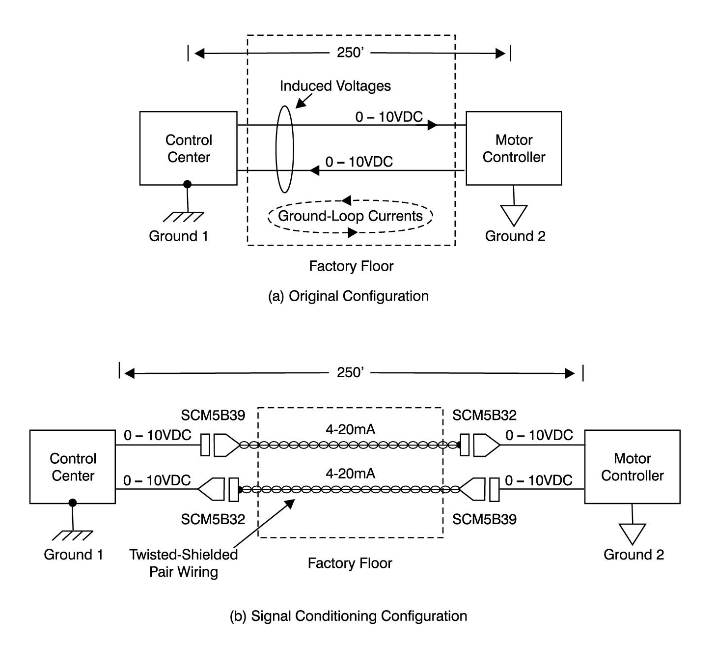 Figure 31: Servo Control Application
The SCM5B32 and SCM5B39 modules provide an additional benefit. Their bandwidth was modified to closely match the dynamic requirements of the control loop. The additional rejection of higher-frequency noise greatly reduced the erratic positioning problems while still providing sufficiently fast response time to provide accurate feedback control.
The changes in control and feedback signals needed to create the incremental movements required at the work piece are extremely small. Some isolation amplifiers can introduce extra noise into the signal path. Isolation amplifiers operate by passing a signal through some non-resistive media to the output. This media may be optical, magnetic or capacitive. Each of these methods makes use of a carrier signal which is modulated by the input signal and transmitted across the isolation media. The signal is then demodulated to produce the output signal. This process can introduce substantial noise and carrier ripple unless carefully controlled by the design of the isolation scheme.
Dataforth’s SCM5B modules are specifically designed to provide extremely low levels of output noise and ripple, providing the high degree of signal integrity required for this application. Additionally, by matching the full-scale signal levels of the original equipment, the SCM5B32 and SCM5B39 modules preserve the signal-to-noise ratio (SNR) of the system.
ALUMINUM SMELTING
The electrolytic production of aluminum takes place in reduction cells or pots. There may be 1,000 or more cells in a modern plant. The reduction cells are made of steel with a carbon lining. Generally, two rows of carbon anodes are suspended overhead from bus bars, which carry the electric power.
The cells are filled with molten cryolite maintained at a temperature of about 980°C by passing direct current through the cells. Alumina is continuously added to the cells. The electric current passing through the cells drives off the oxygen atoms in the alumina, leaving the aluminum atoms to collect as molten aluminum at the bottoms of the cells. Periodically the molten aluminum is drained off. The oxygen atoms adhere to the carbon anodes and gradually erode them. Spent anodes are removed and replaced on a regular schedule. Controlling the electrolysis at the cells and determining when to replace the electrodes are two major problems facing the plant operators.
Normally, the cells operate at about four to six volts drop across the electrodes. Electrical current through the cells ranges from 50,000 to more than 150,000 amperes. The condition of the electrodes can be inferred from the nature of the voltage drop across each cell. The process is controlled by adjusting the immersion depth of the electrodes in response to voltage changes across each cell. High resolution (1mV) is required to maintain good control. However, the chemical activity and deterioration of the electrodes of the electrodes produces electrical noise. Additionally, the high supply voltages present require that the measuring apparatus withstand up to 1500V common-mode voltages. These measurement problems suggest an isolation amplifier with high common-mode rejection, low output noise, good resolution and linearity. The presence of a very sharp low-pass filter response is needed to reduce the undesired electrode noise. Because of the need to resolve 1mV in the presence of common-mode voltages as high as 1500V, the same considerations of low output noise and ripple apply to this measurement problem as existed in the previous servo control application. The Dataforth SCM5B31 provids the right solution for this difficult but crucial measurement problem (Figure 32: Aluminum Smelting Application).
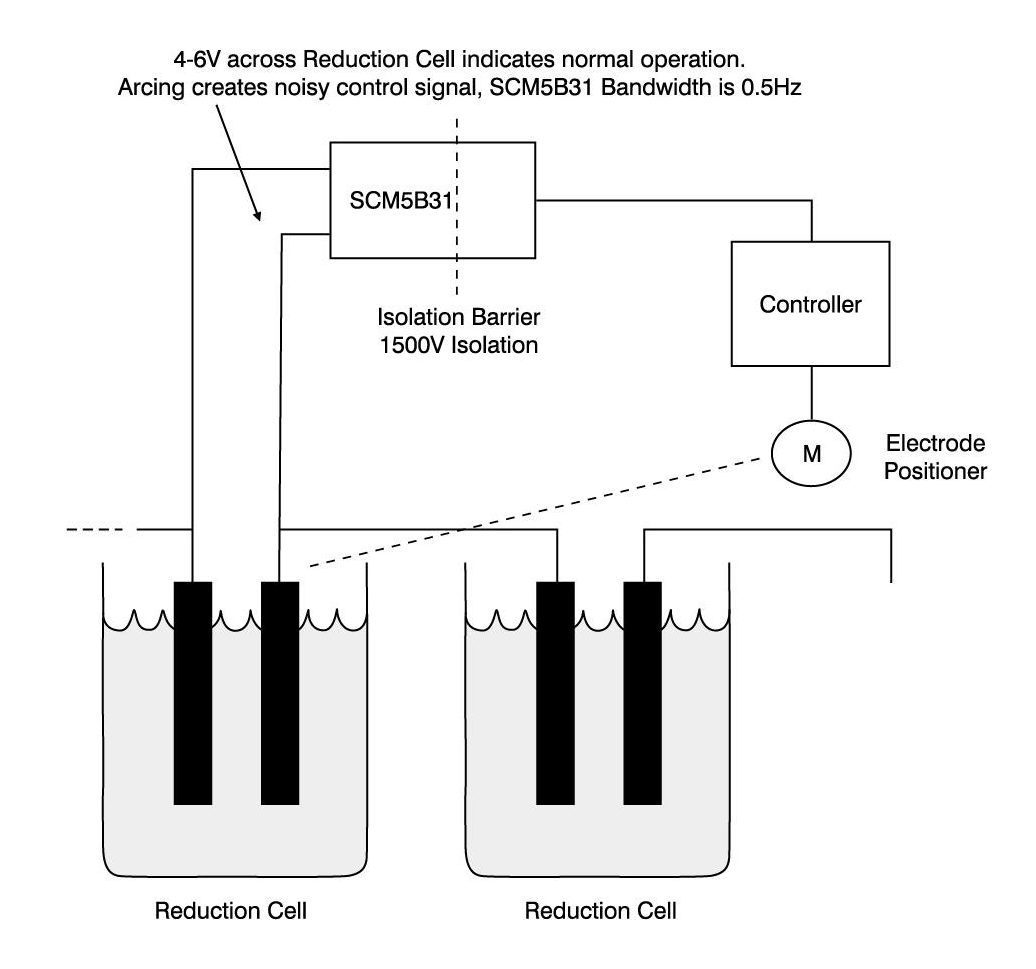 Figure 32: Aluminum Smelting Application
To preserve the benefits obtained with the SCM5B31, care in routing the signal wiring, placement of the signal conditioning equipment and use of twisted, shielded signal wires was of utmost importance. The magnetic and electrical fields surrounding the power busses are quite high and can produce substantial normal-mode error voltages if not properly accounted for. As in most instances, the installation practices are as important as using signal-conditioning equipment with the right characteristics.
GROUNDED THERMOCOUPLES
Some thermocouples used in process-control are made in a unique way. Figure 33: Grounded Thermocouple Application shows this construction. The dissimilar metals are assembled in a concentric arrangement, with a ceramic insulator separating them. They are welded together at the end to form a junction. This provides an extremely robust thermocouple, but the assembly is designed for insertion into a thermo-well — a metal fitting on the vessel that allows removal of a TC or RTD without spilling the vessel’s contents. A thermo-well is always grounded and causes the grounding of this type of thermocouple (Figure 33: Grounded Thermocouple Application).
As explained earlier, shielding and grounding are two of the most difficult problems to deal with. The TC is a low-level signal device and shielding is required. The signal conditioning system has its own ground and the TC is grounded as well. Ground loop potentials and currents are a major problem for this thermocouple type.
There is one completely satisfactory way to solve these problems — insert an isolation stage between the signal and the rest of the measurement system. Note that the isolated signal common can be connected to the signal shield because it is not connected to another earthed ground point, so no ground loop is created. Signal amplification and linearization should take place before the signal is input to the measurement system in order to preserve signal integrity and relax overhead requirements. The TC’s are usually attached to large thermal masses such as storage tanks and therefore do not change output rapidly. A low-bandwidth signal path further reduces noise introduced by the TCs connection to the plant process. An SCM5B47 linearized TC input module selected for the appropriate TC type and temperature range is an optimum choice of signal conditioning for this application (Figure 33: Grounded Thermocouple Application).
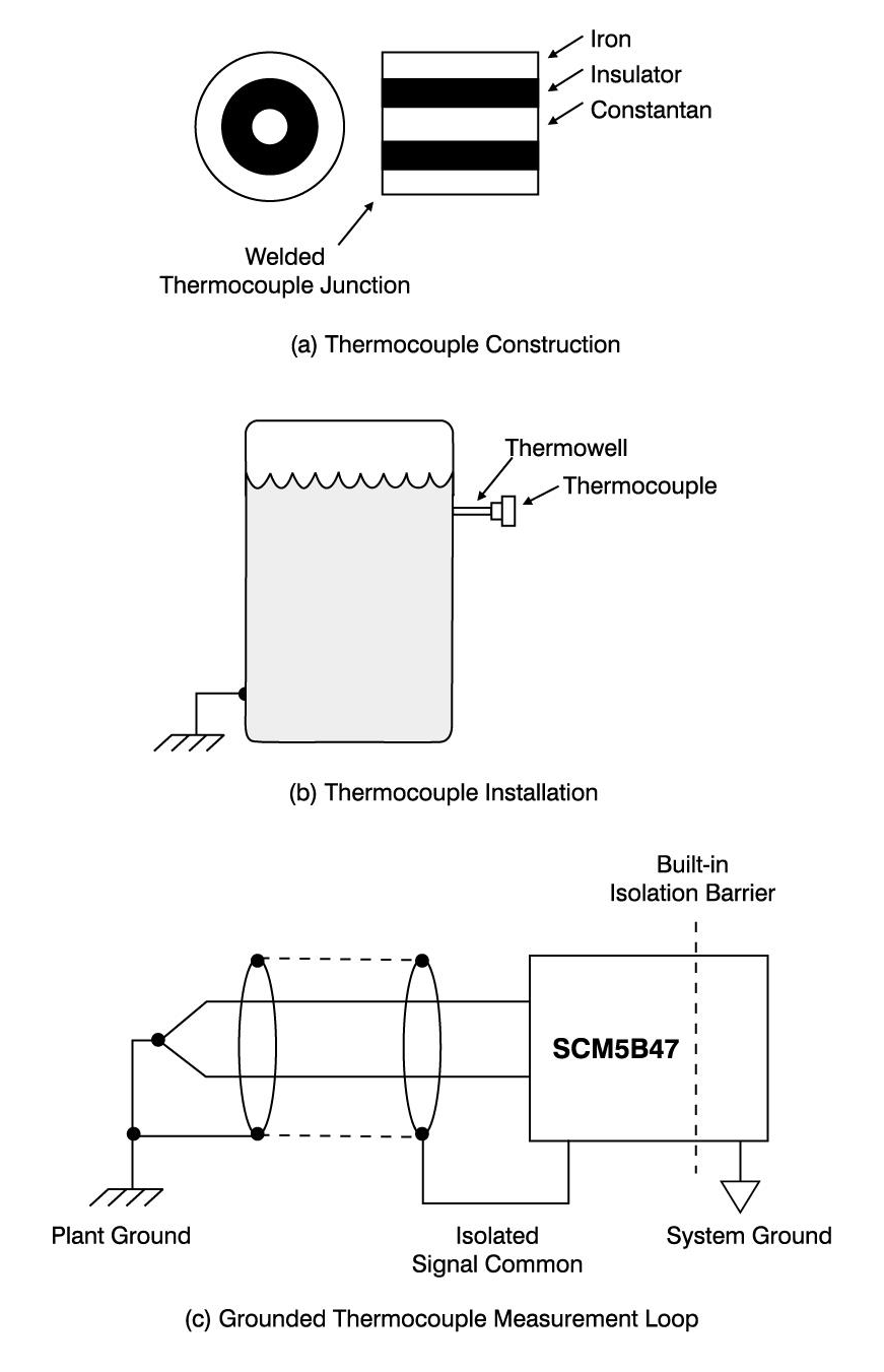 Figure 33: Grounded Thermocouple Application
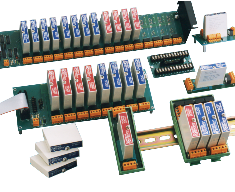
PRODUCT SELECTION GUIDE
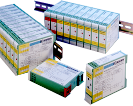
Analog-to-Analog Signal Conditioning Modules
Dataforth was established in 1984 to provide signal conditioning, data acquisition, and data communication hazard protection solutions to the ever-enlarging factory automation markets. The original entrepreneurial venture was spawned by the Burr-Brown Corporation, an international leader in analog integrated circuits and related products and now part of Texas Instruments, Inc. Today, Dataforth is a worldwide innovator of signal conditioning, data acquisition, and data communication products. It maintains a positive revenue growth and delivers a steady introduction of new products offering customers high quality solutions for their industrial applications.
Key Features and Specifications
- 1500Vrms Isolation
- Accuracy, ±0.02 to 0.05% typ
- CMR to 160dB
- NMR to 85-95dB (60Hz)
- Transient Protection, ANSI/IEEE C37.90.1
- Low Output Noise
- CE Compliant to European Emissions and Immunity standards
- CSA C/US certified for safe operation in Class I, Division 2, Groups A, B, C, and D hazardous environments.
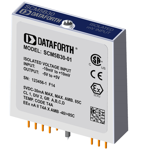
For a list of available SCM5B module products, please visit https://www.dataforth.com/scm5b-signal-conditioner
SCM7B Isolated Process Control Signal Conditioning Modules
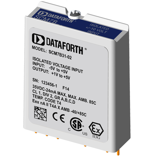
For a list of available SCM7B module products, please visit https://www.dataforth.com/scm7b-signal-conditioner
8B SensorLex® Isolated Analog Signal Conditioning Modules
For a list of available 8B SensorLex® module products, please visit https://www.dataforth.com/8b-signal-conditioner
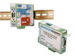
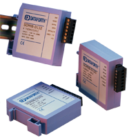
DSCA High Performance DIN-Mount, Isolated Signal Conditioners
For a list of available DSCA products, please visit https://www.dataforth.com/dsca-DIN-rail-signal-conditioner
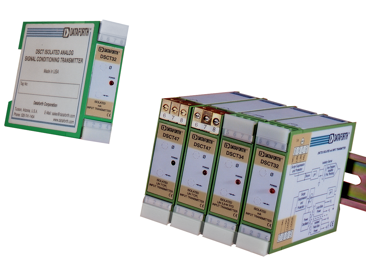
DSCT Isolated Process Control Signal Conditioning Modules
For a list of available DSCT module products, please visit https://www.dataforth.com/dsct-DIN-2-wire-transmitter
Low Cost Industrial Loop Isolators and Programmable Transmitters
The DSCL and DSCP products are a complete family of loop or universal AC/DC powered models of isolators and transmitters in component, DIN and head-mount packages offering fixed-gain or hardware and software programmability. Depending on the model, they accept a wide range of voltage, current, thermocouple, or RTD signals then filter, isolate, amplify, linearize, and convert these input signals to high level analog outputs suitable for use in data acquisition, test and measurement, and control systems.
Key Features and Specifications
- Isolation Protection to 4000Vrms
- DIN, Component, Panel or Instrument Packages
- Signal-Powered Passive Loop Isolators
- 24-60V or 85-230V AC/DC Powered
- Jumper and Software Programmable Models
- Single and Multi-Channel / Splitter Models
- Input Signal Fault Detection Available Models
For a list of available DSCL module products, please visit https://www.dataforth.com/dscl-loop-isolators-and-transmitters
DSCP and SCTP Software Programmable Transmitters
For a list of available DSCP and SCTP module products, please visit https://www.dataforth.com/dscp-sctp-loop-isolators
Industrial and Process Two-wire Transmitters
Dataforth DSCT DIN rail mount isolated, instrument class 2-wire transmitters are low cost, high performance solutions for conditioning and sending analog signals from field sensors to monitoring and control equipment located thousands of feet away in central control areas. They operate on power from a 2-wire output signal loop, modulating the supply current to represent the input signal within a 4 to 20 milliamp range. These transmitters accept a wide range of inputs, and the 4-20mA signal is virtually immune to noise pick-up and interference.
Key Features and Specifications
- Only low-cost, twisted-pair wiring is needed, operates with 10.8V to 100V loop supply voltages
- 1500Vrms transformer isolation
- Input/output protected to 240VAC continuous
- 95dB NMR (60Hz)
- ± 0.05% accuracy
- Panel and DIN mounting options
- CE Compliant to European Emissions and Immunity standards
- CSA C/US certified for safe operation in Class I, Division 2, Groups A, B, C, and D hazardous environments.
For a list of available DSCT products, please visit https://www.dataforth.com/dsct-DIN-2-wire-transmitter
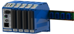
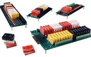
Distributed Data Acquisition and Control Solutions
High quality SCM9B modules provide cost-effective protection and conditioning for a wide range of valuable industrial control signals and systems. Our extensive line includes fixed and programmable sensor-to-computer and computer-to-analog output interface modules, RS-232/RS-485 converters, RS-485 repeaters, and associated backplanes, accessories, and applications software. SCM9B modules are excellent solutions for distributed data acquisition applications such as process monitoring and control, remote data logging, product testing, and motion and motor speed control.
Key Features and Specifications
- 500Vrms input isolation
- Programmable scaling and linearization
- ASCII command/response protocol
- 15-bit measurement resolution
- Continuous self-calibration
- Analog readback
- CE Compliant to European Emissions and Immunity standards
For a list of available SCM9B module products, please visit https://www.dataforth.com/scm9b-signal-conditioner
Industrial Communication Products
Industrial LANs and data communications systems stretch over long distances, inside and outside, with signals exposed to electrical transients, noise, ground loops, power surges, and lightning. Commercial communications equipment often is not designed for use in these environments, which can lead to unreliable signal quality, damage to expensive computers and other online equipment, and production downtime. Our heavy duty modems "harden" and protect these systems, and can extend communications for many miles without expensive cabling.
Key Features and Specifications
- Protects equipment from damage due to power surges, transients, lightning
- 1500Vrms isolation with opto couplers and power DC-to-DC converter (6000VDC, 1 min)
- Extends RS-232 communications distances without expensive low capacitance cabling
- Connects RS-232 devices to RS-422 and RS-485 devices
- Data rates to 115K Baud
- Distances to 12 miles (20Km)
- CE Compliant to European Emissions and Immunity standards
For a list of available LDM Series products, please visit https://www.dataforth.com/Modular_Converters_Line_Drivers.aspx
DCP Series—DIN Rail Mount Industrial Data Products
For a list of available DCP Series products, please visit https://www.dataforth.com/din_rail_converters_line_drivers.aspx